Week 4.1 - Genetic Algorithm

- Objectives:

• To write a code in MATLAB to optimise the stalagmite function and find the global maxima of the function.
• To clearly expalin the concept of genetic algorithm in your own words and also explain the syntax for ga in MATLAB in the report.
• To make sure that the code gives the same output, even if it is made to run several times.
• To plot graphs for all 3 studies and for F maximum vs no. of iterations. Title and axes labels.

- Function Code is shown below:

function [f] = stalagmite(V)

x= V(1);
y= V(2);


f1x= (sin((5.1*pi*x)+0.5))^6;
f1y= (sin((5.1*pi*y)+0.5))^6;
f2x= exp(-4*log(2)*(((x-0.0667)^2)/0.64));
f2y= exp(-4*log(2)*(((y-0.0667)^2)/0.64));


f= - (f1x*f1y*f2x*f2y);

end

- Program code is shown below:

clear all
close all
clc


% defining the space of the objective function

x = linspace(0,0.6,200);
y=  linspace(0,0.6,200);

[xx,yy] = meshgrid (x,y);

%Evaluating the objective function

for i = 1:length(x)
    for j = 1:length(y)

        inputs(1)= xx(i,j);
        inputs(2)= yy(i,j);
        f(i,j)= stalagmite(inputs);
    end
end


figure(1)
surfc(x,y,-f)
xlabel('x-values')
ylabel('y-values')
zlabel('z-values')
shading interp



% study-1: Unbounded GA 

for i= 1:50

    [input,fopt(i)] = ga(@stalagmite,2);
    xopt(i) = input(1);
    yopt(i) = input(2);

end

figure(2)
subplot(2,1,1)
surfc(x,y,-f)
xlabel('x')
ylabel('y')
shading interp

hold on

plot3(xopt,yopt,-fopt, 'Marker','.','MarkerSize',5)
title('Study-1: Unbounded GA')


subplot(2,1,2)
plot(-fopt)
xlabel('Iteration')
ylabel('function maximum value')


% study-2: Bounded GA

for i = 1:50

    [input,fopt(i)] = ga(@stalagmite,2,[],[],[],[],[0;0],[0.4;0.4]);
    xopt(i) = input(1);
    yopt(i) = input(2);

end
figure(3)

subplot(2,1,1)
surfc(x,y,-f)
xlabel('x')
ylabel('y')
shading interp

hold on

plot3(xopt,yopt,-fopt, 'Marker','.','MarkerSize',5)
title('Study-2: Bounded GA')


subplot(2,1,2)
plot(-fopt)
xlabel('Iteration')
ylabel('function maximum value')



% study-3: Bounded GA with population size

% returns a set of default options for the solverName solver
options = optimoptions('ga');

% Defining population size
options = optimoptions(options,'PopulationSize',270);

for i = 1:50

    [input,fopt(i)] = ga(@stalagmite,2,[],[],[],[],[0;0],[0.4;0.4],[],[],options);
    xopt(i) = input(1);
    yopt(i) = input(2);
end

figure(4)

subplot(2,1,1)
surfc(x,y,-f)
xlabel('x')
ylabel('y')
shading interp

hold on

plot3(xopt,yopt,-fopt, 'Marker','.','MarkerSize',5)
title('Study-3: Bounded GA with increasing population size')


subplot(2,1,2)
plot(-fopt)
xlabel('Iteration')
ylabel('function maximum value')

-Global Maxima Plot:

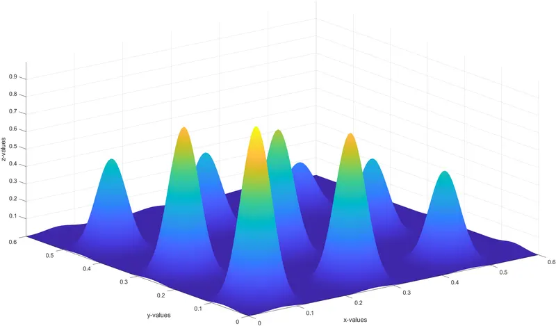
-Study-1: Unbounded GA plot:

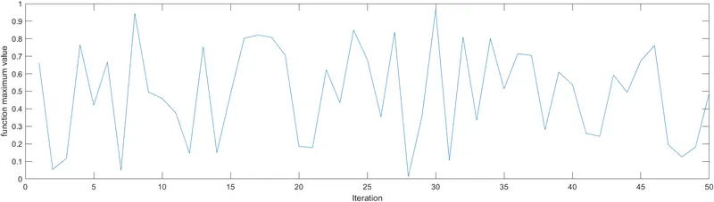
- Study-2: Bounded GA plot :

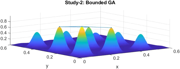
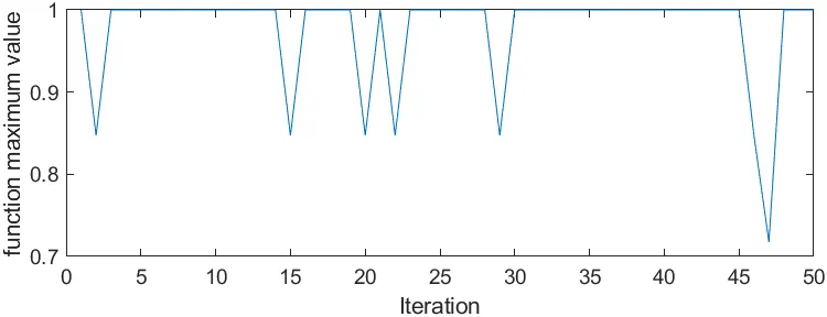
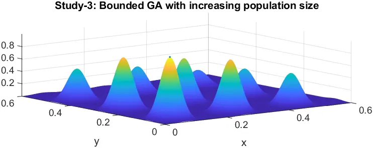
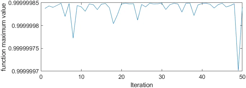
- Study-3: Bounded GA with increased population size Plot:

GA syntax:

x= ga (fun, nvars, A , b , Aeq, Beq, lb,up, nonlcon,options)

where:

fun : objective function

nvar: number of variables

A,b : linear inequality constrains

Aeq, beq : linear equality constrains.

lb,up: lower bounds and upper bounds.

nonlcon: Non-linear constains.

options: optimization options.

Explaination of codes:

In the function code, the function describes the stalagmite function which creates the contour of peaks for the defined input variables with suitable range.In addition, it is also known as a test function which is used to validate the performance characteristics of the optimization algorithms.

In the program code shown above, I have defined the input space for the possible range of inputs. this input will be considered as the space for the algorithm to solve. After that, I have used a for loop to cover the two dimensional input x and y, so that sor each point in the xy plane stalagmite function will be called to calculate f value.

for study-1 which is unbounded GA study, the lower and upper bounds were not defined resulting for getting inaccurate results as the plot has shown.

for study-2 which is bounded GA study, the lower and upper bounds were defined form 0 to o.4 for each x and y bounds resulting in getting better optimization.

for study-3 which is bounded GA study with increasing the population size, the lower and upper bounds were defined in addition, the population sized was increased to 270.

the command 'optimoptions' was used to define the population size, and the default population size for ga solver is 50.

increasing the population size is helpful in order to achieve the single optimum point as well as the simulation time.