Week 4.1 - Genetic Algorithm

Theory:

Nature has always been a great source of inspiration to all mankind. Genetic Algorithms (GAs) are search based algorithms based
on the concepts of natural selection and genetics. GAs are a subset of a much larger branch of computation known as Evolutionary
Computation.
GAs were developed by John Holland and his students and colleagues at the University of Michigan, most notably David E. Goldberg
and has since been tried on various optimization problems with a high degree of success.
In GAs, we have a pool or a population of possible solutions to the given problem. These solutions then undergo recombination and
mutation (like in natural genetics), producing new children, and the process is repeated over various generations. Each individual
(or candidate solution) is assigned a fitness value (based on its objective function value) and the fitter individuals are given a
higher chance to mate and yield more “fitter” individuals. This is in line with the Darwinian Theory of “Survival of the Fittest”.
In this way we keep “evolving” better individuals or solutions over generations, till we reach a stopping criterion.
Genetic Algorithms are sufficiently randomized in nature, but they perform much better than random local search (in which we just
try various random solutions, keeping track of the best so far), as they exploit historical information as well.

Aim

To write code to calculate Global Maxima using Genetic Algorithm, using MATLAB.

PROCEDURE:
The stalagmite function is defined separately. This function is later called into the main GA program.
Now we define the x and y inputs using linspace command.
Then the input vectors are transformed into array [xx,yy], so that it can be used to evaluate the functions of two variables and plot
three-dimensional mesh/surface plots.
Now the values in the different matrix created can be put as an input into the function that we have created, by calling it. By
this we can get the value of the stalagmite function at various values of x and y.
Now since we have got the value of the function at various values, we now need to calculate the maxima value, which can be
calculated using the ga command, which is an in-built function in MATLAB.
Then, the total number of times the ga needs to run is defined using num_cases, and with help of for loop ga is made to run for
each iteration and the value is stored in an array.
GA generally gives the minima value(in built-in MATLAB), but we need the maxima hence we can just inverse the stalagmite
function by introducing a 'Negative sign'(This inverses the stalagmite curve and the Global maxima can be found, instead
minima)
The total study time is calculated using the 'tic' and 'toc' commands at the start and end of the ga for loop respectively.
The results are then plotted using the surf command and plot command.
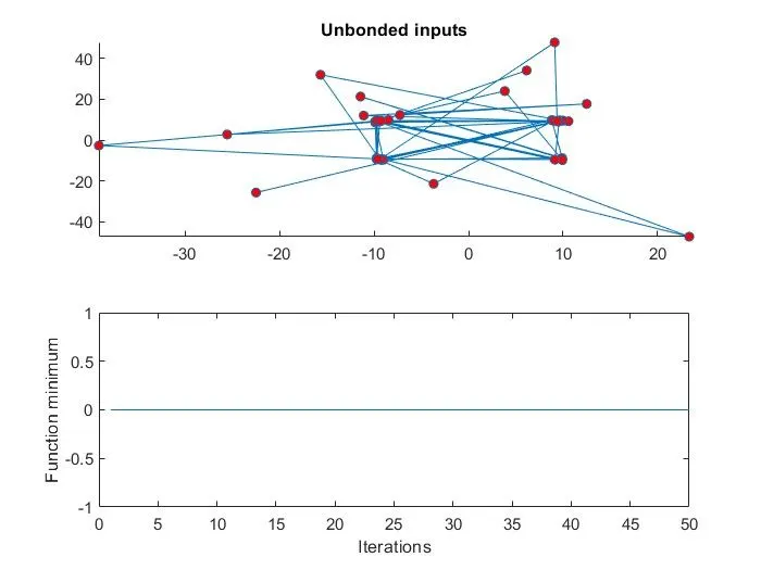
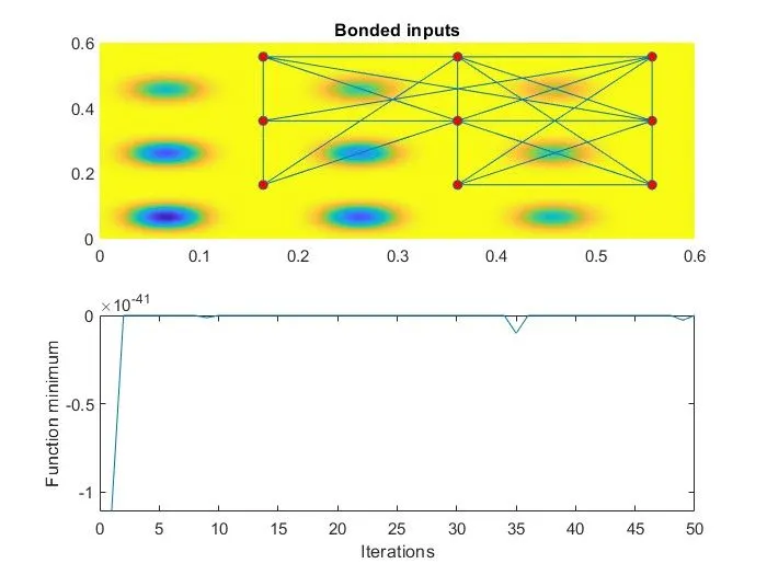
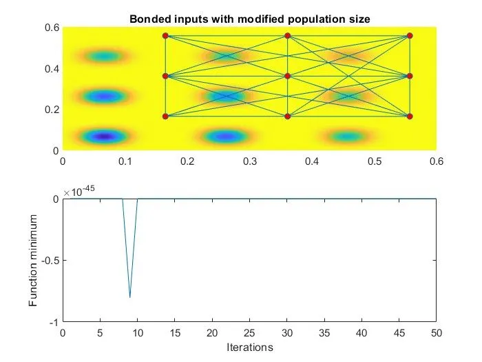
GA is made to run for 3 iterations, with each iteration having bounded inputs, unbounded inputs, and increasing population
size.

clear all
close all
clc

x = linspace(0,0.6,150);
y = linspace(0,0.6,150);

num_cases = 50


% Creating a 2Dimensional mesh
[xx,yy] = meshgrid(x,y)


% Logic
for i = 1:length(xx)
for j = 1:length(yy)
input_vector(1) = xx(i,j);
input_vector(2) = yy(i,j);
f(i,j) = stalagmite(input_vector);
end
end
 tic
% Study 1 - Satistical behaviour
for i = 1:num_cases
    [inputs, fopt(i)] = ga(@stalagmite, 2);
    xopt(i) = inputs(1);
    yopt(i) = inputs(2);
end

study_time = toc

figure(1)
subplot(2,1,1)
hold on
surfc(x, y, -f)
shading interp
plot3(xopt,yopt,-fopt,'marker','o','markersize',5,'markerfacecolor','r')
title('Unbonded inputs')
subplot(2,1,2)
plot(-fopt)
xlabel('Iterations')
ylabel('Function minimum')

tic
% Study 2 - Stastical behaviour - with upper & lower bounds
for i = 1:num_cases
    [inputs, fopt(i)] = ga(@stalagmite,2,[],[],[],[],[0;0],[0.6;0.6]);
    xopt(i) = inputs(1);
    yopt(i) = inputs(2);
end
study2_time = toc

figure(2)
subplot(2,1,1)
hold on
surfc(x, y, -f)
shading interp
plot3(xopt,yopt,-fopt,'marker','o','markersize',5,'markerfacecolor','r')
title('Bonded inputs')
subplot(2,1,2)
plot(-fopt)
xlabel('Iterations')
ylabel('Function minimum')

% Study 3 increaing GA iterations
options = optimoptions('ga');
options = optimoptions(options,'PopulationSize', 170);


tic
for i = 1:num_cases
    [inputs, fopt(i)] = ga(@stalagmite,2,[],[],[],[],[0;0],[0.6;0.6],[],[],options);
    xopt(i) = inputs(1);
    yopt(i) = inputs(2);
end

study3_time = toc
figure(3)
subplot(2,1,1)
hold on
surfc(x, y, -f)
shading interp
plot3(xopt,yopt,-fopt,'marker','o','markersize',5,'markerfacecolor','r')
title('Bonded inputs with modified population size')
subplot(2,1,2)
plot(-fopt)
xlabel('Iterations')
ylabel('Function minimum')

function f =  stalagmite(input_vector)

x = input_vector(1);
y = input_vector(2);

f1 = ((sin(5.1*pi*x+0.5)))^6;
f2 = ((sin(5.1*pi*y+0.5)))^6;
f3 = exp(-4*log(2)*((x-0.0667)^2/0.64));
f4 = exp(-4*log(2)*((y-0.0667)^2/0.64));

f = (f1*f2*f3*f4);
end