Week 4.1 - Genetic Algorithm

AIM:

To write a MATLAB code that solves the stalagmite function and finds the same global maxima.

Genetic Algorithm:

• Genetic Algorithm is one of the search-based optimization technique based on the principles of genetics and natural selection.GA is basically the process of selecting the best solution for the group or population.
• The structure of GA is as follows,

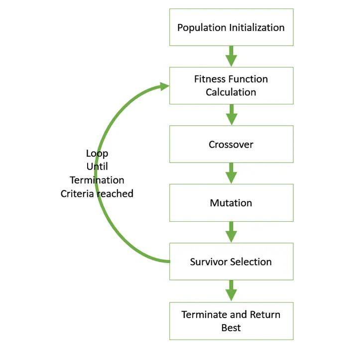
• Simply, GA is the process of selecting the population from which the best optimum results is to be obtained. Then, from the group, fitness individuals are selected who are better than other individuals for producing best offspring. Then, Among the selected fitness value, parents are selected for producing the output. Crossover method is used where two or more parents are considered for producing multiples offsprings and Mutation method is where changes are made in individuals to get optimal value.
• Survivor selection is where fitter individuals are kept and other individuals are removed from the process to avoid improper combination.
• Termination condition has to be used as GA keeps processing for multiple itertaions. The same process has been repeated until optimum results are obtained.

GA Syntax:

x= ga(fun,nvars,A,B,[],[],lb,ub,nonlcon,IntCon,options)

x= local minima point.

fun-calling function.

nvars - no. of variables

A & B - Inequalities

lb & ub - Lower bound and Upper bound.

nonlcon - vectors representing equalities and inequalities

options - for performing additional operations like increasing population.

MATLAB code:

Fitness calling function to be used in the main function:

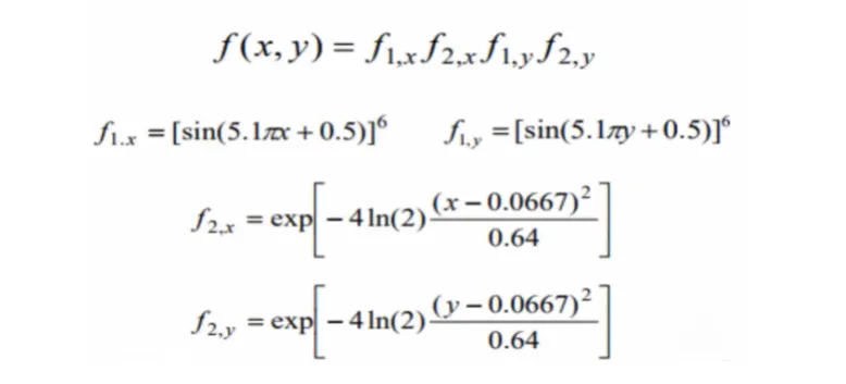
function[f]= stalagmite(input_vector)

x= input_vector(1);
y=input_vector(2);

f1=(sin(5.1*pi*x +0.5)).^6;
f2=(sin(5.1*pi*y +0.5)).^6;

f3=exp((-4*log(2)*(x-0.0667).^2)/(0.64));
f4=exp((-4*log(2)*(y-0.0667).^2)/(0.64));

f=-f1*f2*f3*f4;

end

• In the above code, - symbol is used to find the global maxima as GA generally find the local minima.

MATLAB code:

clear all
close all
clc

%Defining the search space

x=linspace(0,0.6,150);
y=linspace(0,0.6,150);
num_cases=50;
[xx yy]= meshgrid(x,y);

%Stalagmite func

for i= 1: length(xx);
    for j= 1:length(yy);
        input_vector(1)= xx(i,j);
        input_vector(2)=yy(i,j);
        f(i,j)=stalagmite(input_vector);
    end
end

surfc(xx,yy,f)
shading interp

%Study 1 statistical behaviour
tic

for i=1:num_cases;
    [inputs,f_opt(i)]=ga(@stalagmite,2);
    x_opt(i)=inputs(1);
    y_opt(i)=inputs(2);
    
end
study_time1=toc

%plotting study_time1

figure(1)
subplot(2,1,1)
hold on
surfc(xx,yy,f)
shading interp
plot3(x_opt,y_opt,f_opt,'marker','o','markersize',5,'markerfacecolor','r')
title('Unbouned Inputs')
xlabel('xvalue')
ylabel('yvalue')
subplot(2,1,2)
plot(f_opt)
xlabel('Iterations')
ylabel('Function Max')
%Study 2 - statiscal behaviour with upper and lower bounds

tic

for i=1:num_cases;
    [inputs,f_opt(i)]=ga(@stalagmite,2,[],[],[],[],[0;0],[1;1]);
    x_opt(i)=inputs(1);
    y_opt(i)=inputs(2);
    
end
study_time2=toc

%plotting study_time2

figure(2)
subplot(2,1,1)
hold on
surfc(xx,yy,f)
shading interp
plot3(x_opt,y_opt,f_opt,'marker','o','markersize',5,'markerfacecolor','r')
title('Bouned Inputs')
xlabel('xvalue')
ylabel('yvalue')
subplot(2,1,2)
plot(f_opt)
xlabel('Iterations')
ylabel('Function Max')

%Study 2 - statiscal behaviour with upper and lower bounds

tic

for i=1:num_cases;
    [inputs,f_opt(i)]=ga(@stalagmite,2,[],[],[],[],[0;0],[1;1]);
    x_opt(i)=inputs(1);
    y_opt(i)=inputs(2);
    
end
study_time2=toc

%plotting study_time2

figure(2)
subplot(2,1,1)
hold on
surfc(xx,yy,f)
shading interp
plot3(x_opt,y_opt,f_opt,'marker','o','markersize',5,'markerfacecolor','r')
title('Bouned Inputs')
xlabel('xvalue')
ylabel('yvalue')
subplot(2,1,2)
plot(f_opt)
xlabel('Iterations')
ylabel('Function Max')

%Study 3 - Increasing the GA iterations
options=optimoptions('ga')
options=optimoptions(options,'populations',200)
tic

for i=1:num_cases;
    [inputs,f_opt(i)]=ga(@stalagmite,2,[],[],[],[],[0;0],[1;1],[],[],options);
    x_opt(i)=inputs(1);
    y_opt(i)=inputs(2);
    
end
study_time3=toc

%plotting study_time3

figure(3)
subplot(2,1,1)
hold on
surfc(xx,yy,f)
shading interp
plot3(x_opt,y_opt,f_opt,'marker','o','markersize',5,'markerfacecolor','r')
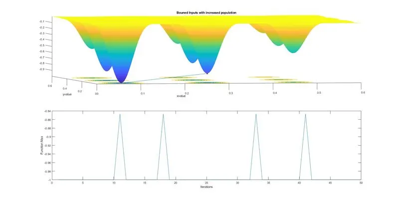
title('Bouned Inputs with increased population')
xlabel('xvalue')
ylabel('yvalue')
subplot(2,1,2)
plot(f_opt)
xlabel('Iterations')
ylabel('Function Max')

Code Explanation:

• Intially, the calling function 'stalagmite' is created.
• Then, on the main function, search space is defined with x and y and values for xx and yy are calculated using meshgrid command.
• The, stalagmite function is called for with respect to the values of i and j as input vectors
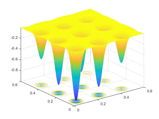
• plot for the stalagmite function is plotted.
• Then, 3 different studies are written to find the best optimum value.
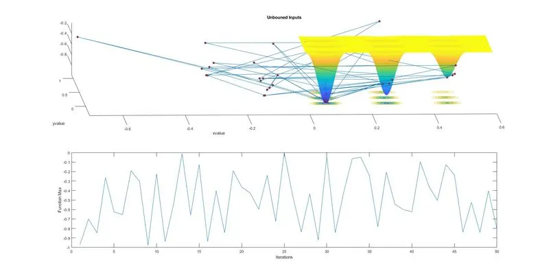
• Study1- statistical behaviour, where general ga syntax is used and plotted.
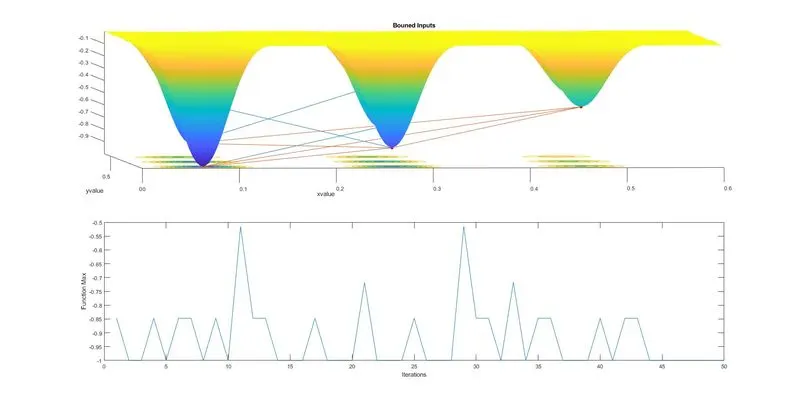
• Study2 - Statistical behaviour with upper and lower bound, where ga syntax with boundary values are set and plotted.
• Study3 - Increaed population size , since GA selects random number between 50 iterations, the population value has been increased and plotted.
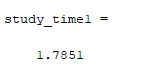
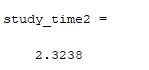
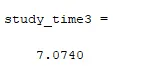
• Time takes for all the studies are mentioned below.

Ouputs:

1. Studytime 1

2. Studytime2

3. Studytime 3

Plots:

Stalagmite function:

1. Studytime 1

2. Studytime 2

3. Studytime 3

Code for evaluation of the population size fitness function:

clear all
close all
clc

%Defining the search space

x=linspace(0,0.6,150);
y=linspace(0,0.6,150);
num_cases=50;
[xx yy]= meshgrid(x,y);

%Stalagmite func

for i= 1: length(xx);
    for j= 1:length(yy);
        input_vector(1)= xx(i,j);
        input_vector(2)=yy(i,j);
        f(i,j)=stalagmite(input_vector);
    end
end



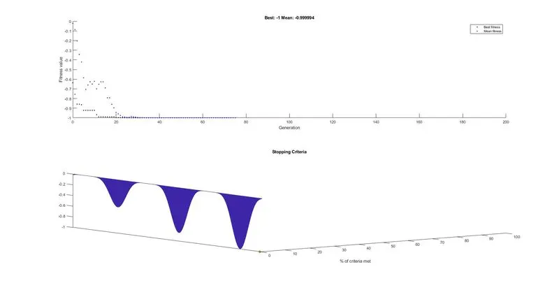
options=optimoptions('ga','plotFcn',{@gaplotbestf,@gaplotstopping},'populationsize',170);
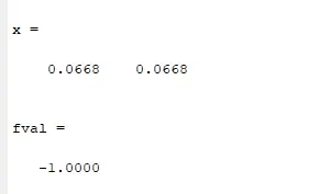
[x,fval]=ga(@stalagmite,2,[],[],[],[],[0;0],[1;1],[],options)

x_opt=x(1);
y_opt=y(2);

figure(1)
surf(xx,yy,f)
shading interp
hold on
plot3(x_opt,y_opt,fval,'ro','markersize',5,'markerfacecolor','g')

Explanation:

Here, fitness function command is used to determine the best value. Plot for the graph is used and plotted and best fitness value is found be around -1.

Output:

Plot:

Conclusion:

From the above program, different studies are conducted for stalagmite function with a Genetic Algorithm.

References used:

1. https://www.tutorialspoint.com/genetic_algorithms/genetic_algorithms_survivor_selection.html

2. https://mech.iitm.ac.in/nspch52.pdf

3. https://in.mathworks.com/help/gads/ga.html#d123e39036

4. https://in.mathworks.com/help/gads/genetic-algorithm-options.html