Week 4.1 - Genetic Algorithm
1. AIM: To write a code in MATLAB to optimize the stalagmite function, find the global maxima of the function, and Plot graphs for all 3 studies and for F maximum vs no. of iterations.
2. THEORY:
2.1 OPTIMIZATION:
Optimization is defined as finding the best solution from the feasible solution in a pool which contains all solutions. In many engineering problems, the optimal solution can be the minimum or maximum value of the objective function of the problem.
2.1.1 OPTIMIZATION TECHNIQUES IN ENGINEERING:
- Optimization IntroductionMathematical Modeling
- Unconstrained Optimization
- Discrete Optimization
- Genetic Algorithm
- Constrained Optimization
- Robust Optimization
- Dynamic Optimization
2.1.2 APPLICATIONS OF OPTIMIZATION IN ENGINEERING:
- structural design (including pressure vessel design and welded beam design)
- shape optimization
- topology optimization (including airfoils)
- inverse optimization (a subset of the inverse problem)
- processing planning
- product designs
- electromagnetic optimization
- space mapping
- aggressive space mapping
- yield-driven design
- optimization exploiting surrogates (surrogate model)
2.2 GENETIC ALGORITHM:
- A genetic algorithm (or GA) is a search technique used in computing to find true or approximate solutions to optimization and search problems.
- (GA)s are categorized as global search heuristics.
- (GA)s are a particular class of evolutionary algorithms that use techniques inspired by evolutionary biologies such as inheritance, mutation, selection, and crossover (also called recombination).
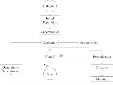
- The evolution usually starts from a population of randomly generated individuals and happens in generations.
- In each generation, the fitness of every individual in the population is evaluated, multiple individuals are selected from the current population (based on their fitness), and modified to form a new population.
- The new population is used in the next iteration of the algorithm.
- The algorithm terminates when either a maximum number of generations has been produced, or a satisfactory fitness level has been reached for the population.
2.2.1 VOCABULARY:
- Individual - Any possible solution
- Population - Group of all individuals
- Fitness function– Target function that we are optimizing (each individual has a fitness)
- Trait - Possible aspect (features) of an individual
- Genome - Collection of all chromosomes (traits) for an
individual.
- The idea of the selection phase is to select the fittest individuals and let them pass their genes to the next generation.
- Two pairs of individuals (parents) are selected based on their fitness scores. Individuals with high fitness have more chance to be selected for reproduction.
CROSSOVER:
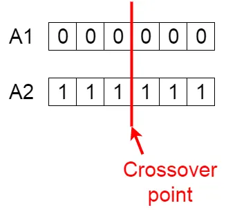
- Crossover is the most significant phase in a genetic algorithm. For each pair of parents to be mated, a crossover point is chosen at random from within the genes. For example, consider the crossover point to be 3 as shown below.
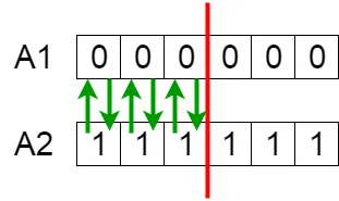
- Offspring are created by exchanging the genes of parents among themselves until the crossover point is reached.
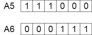
- The new offspring are added to the population.
MUTATION:
- In certain new offspring formed, some of their genes can be subjected to a mutation with a low random probability. This implies that some of the bits in the bit string can be flipped.
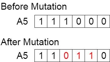
- Mutation occurs to maintain diversity within the population and maintain premature convergence.
TERMINATION:
- The algorithm terminates if the population has converged (does not produce offspring which are significantly different from the previous generation). Then it is said that the genetic algorithm has provided a set of solutions to our problem.
2.2.3 METHODOLOGY:
2.3 GENETIC ALGORITHM IN MATLAB:
2.3.1 SYNTAX:
x = ga(fun,nvars,A,b,Aeq,beq,lb,ub,nonlcon,options)
- ga finds a local minimum
xtofun, subject to the linear inequalitiesA*x≤b.gaevaluates the matrix productA*xas ifxis transposed (A*x'), subject to the linear equalitiesAeq*x=beqandA*x≤b. (SetA=[]andb=[]if no linear inequalities exist.)gaevaluates the matrix productAeq*xas ifxis transposed (Aeq*x'), defines a set of lower and upper bounds on the design variables,x, so that a solution is found in the rangelb≤x≤ub. (SetAeq=[]andbeq=[]if no linear equalities exist.), subjects the minimization to the constraints defined innonlcon. The functionnonlconacceptsxand returns vectorsCandCeq, representing the nonlinear inequalities and equalities respectively.gaminimizes thefunsuch thatC(x)≤0andCeq(x) = 0. (Setlb=[]andub=[]if no bounds exist.) and minimizes with the default optimization parameters replaced by values inoptions. (Setnonlcon=[]if no nonlinear constraints exist.) Createoptionsusing optimoptions.
2.4 STALAGMITE:
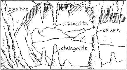
- A stalagmite is a type of rock formation that rises from the floor of a cave due to the accumulation of material deposited on the floor from ceiling drippings. Stalagmites are typically composed of calcium carbonate but may consist of lava, mud, peat, pitch, sand, sinter, and amber.
2.4.1 STALAGMITE MATHEMATICAL MODEL:
3. MATLAB CODE :
3.1. MAIN CODE:
clear all
close all
clc
x=linspace(0,0.6,150);
y=linspace(0,0.6,150);
num_cases=50;

[f ]=get_stalagmite(x,y);

% study1 - statistical behaviour without bounds
for i=1:num_cases
    [inputs fopt(i)]= ga(@stalagmite,2);
    xopt(i)=inputs(1);
    yopt(i)=inputs(2);
end

figure(1)
subplot(2,1,1)
hold
surfc(x,y,f)
shading interp
plot3(xopt,yopt,fopt,'marker','o','markersize',5 ,'markerfacecolor','r')
title('unbounded inputs')


subplot(2,1,2)
plot(fopt)
xlabel('no_of_iterations')
ylabel('minimum_of_function')


% study 2 - statistical behaviour with lower and upper bounds
for i=1:num_cases
    [inputs fopt(i)]= ga(@stalagmite,2,[],[],[],[],[0,0],[1,1]);
    xopt(i)=inputs(1);
    yopt(i)=inputs(2);
end

figure(2)
subplot(2,1,1)
hold
surfc(x,y,f)
shading interp
plot3(xopt,yopt,fopt,'marker','o','markersize',5 ,'markerfacecolor','r')
title('bounded inputs')


subplot(2,1,2)
plot(fopt)
xlabel('no_of_iterations')
ylabel('minimum_of_function')


%study 3 - increasing ga iterations by increasing population size
options = optimoptions(@ga,'PopulationSize',300);

for i=1:num_cases

    [inputs fopt(i)]= ga(@stalagmite,2,[],[],[],[],[0,0],[1,1],[],[],options);
    xopt(i)=inputs(1);
    yopt(i)=inputs(2);
end

figure(3)
subplot(2,1,1)
hold
surfc(x,y,f)
shading interp
plot3(xopt,yopt,fopt,'marker','o','markersize',5 ,'markerfacecolor','r')
title('increased population size')


subplot(2,1,2)
plot(fopt)
xlabel('no_of_iterations')
ylabel('minimum_of_function')
3.2 GET STALAGMITE FUNCTION CODE:
function [f xx yy]=get_stalagmite(x,y)
[xx yy]=meshgrid(x,y);

for i = 1:length(xx)
    for j=1:length(yy)
        a(1)=xx(i,j);
        a(2)=yy(i,j);
        f(i,j) =stalagmite(a);
    end
end
3.3 STALAGMITE FUNCTION CODE:
function [f]=stalagmite(a)
    x=a(1);
    y=a(2);
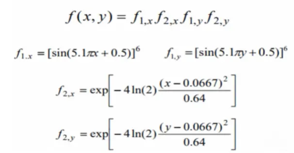
    f1x=(sin((5.1*pi.*x )+0.5)).^6;
    f1y=(sin((5.1*pi*y)+0.5)).^6;
    a1=-4*log(2).*((x-0.0667).^2 )/0.64;
    a2=-4*log(2).*((y-0.0667).^2) /0.64;
    f2x=exp(a1);
    f2y=exp(a2);
    f=-(f1x.*f1y.*f2x.*f2y);
end
4. OBSERVATIONS:
PLOT 1
PLOT 2
PLOT 3
5. CONCLUSION:
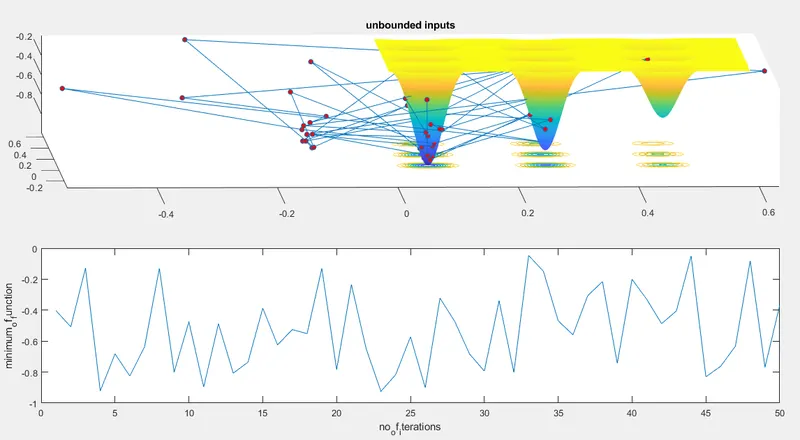
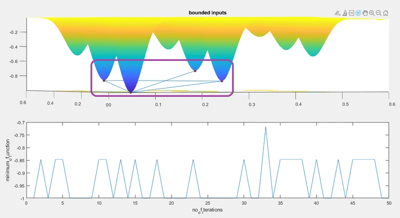
- CASE 1: From plot 1, it is observed that the output predicted by the genetic algorithm is not the same in every iteration. Because genetic algorithm deals with the random sampling of the population. The sample population would be different in each iteration. ga finds the best solution in the given sample of the population only. so that the different outputs are obtained.
- CASE 2: In the second plot, it is found that the efficiency of the ga has been increased with bounded inputs. So that accuracy is more than that of the case with unbounded inputs.
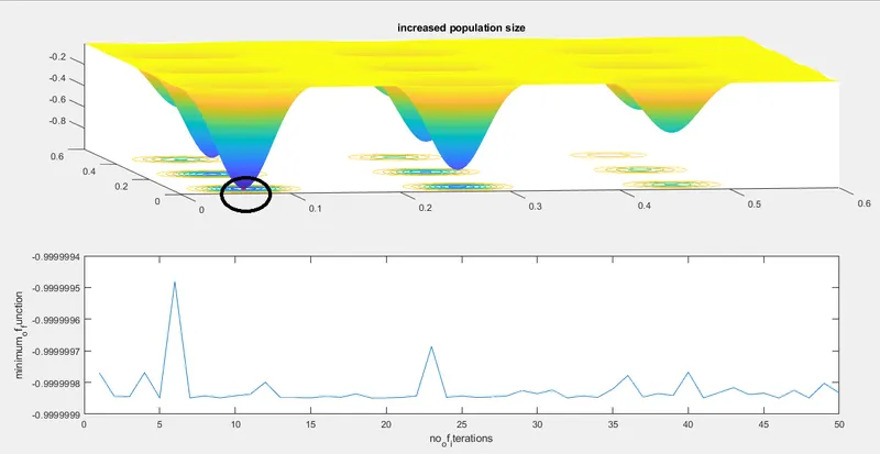
- CASE 3: In the third study, the accuracy of the genetic algorithm is improved as expected, since the population size is increased. Because the number of sample data points taken by the ga is gone up.
6. REFERENCES:
- https://in.mathworks.com/help/gads/how-the-genetic-algorithm-works.html
- https://skill-lync.com/knowledgebase/genetic-algorithm-explained
- https://in.mathworks.com/help/gads/ga.html
- https://in.mathworks.com/help/gads/options-in-genetic-algorithm.html
- https://in.mathworks.com/help/gads/genetic-algorithm-options.html
- https://www.iitg.ac.in/rkbc/CE602/CE602/Genetic%20Algorithms.pdf
- https://www.linkedin.com/pulse/introduction-optimization-genetic-algorithm-ahmed-gad