Week 3 - Solving second order ODEs

1. AIM: To write a program that solves the ODE which represents the equation of motion of a simple pendulum with damping.

2. THEORY:

2.1 IMPORTANCE OF ODE IN ENGINEERING:

• In engineering and science, a differential equation is a mathematical formulation of a physical law formulated in terms of rates of change (i.e. derivatives) of some physical quantities.
• The solution of a differential equation is not unique (It contains arbitrary constants). It is a natural reflection of the fact that a physical law describes an infinitely large number of processes.
  
• In order to obtain a unique process, a unique solution of a differential equation, we need to use additional conditions, e.g., we need to fix initial conditions, i.e. specify the initial state of the process.
  
• The number of initial conditions (parameters that we need to fix at the initial time) coincides with the highest derivative in the equation.

2.2 ENGINEERING APPLICATIONS OF ODE:

• Differential equations have wide applications in various engineering and science disciplines. In general, modeling of the variation of a physical quantity, such as temperature, pressure, displacement, velocity, stress, strain, current, voltage, or concentration of a pollutant, with the change of time or location, or both would result in differential equations. Similarly, studying the variation of some physical quantities on other physical quantities would also lead to differential equations.
  
• In fact, many engineering subjects, such as mechanical vibration or structural dynamics, heat transfer, or the theory of electric circuits, are founded on the theory of differential equations. It is practically important for engineers to be able to model physical problems using mathematical equations, and then solve these equations so that the behavior of the systems concerned can be studied.
  

2.3 SIMPLE PENDULUM:

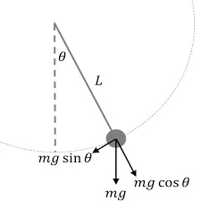
FIGURE 1

• A pendulum is a weight suspended from a pivot so that it can swing freely.
  
• When a pendulum is displaced sideways from its resting, equilibrium position, it is subject to a restoring force due to gravity that will accelerate it back toward the equilibrium position. When released, the restoring force acting on the pendulum's mass causes it to oscillate about the equilibrium position, swinging back and forth.
  
• The time for one complete cycle, a left swing and a right swing is called the period. The period depends on the length of the pendulum and also to a slight degree on the amplitude, the width of the pendulum's swing.
  

2.4 APPLICATIONS OF SIMPLE PENDULUM:

• Clock
  
• Car Shock Absorbers
  
• Musical Instruments
  
• Bungee Jumping
  
• Diving Board
  
• The Process of Hearing
  
• Earthquake-proof buildings
  
• Metronome
  

2.5 ODE OF SIMPLE PENDULUM WITH DAMPING:

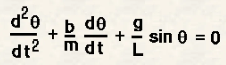
In the above equation,

g = gravity in m/s2,

L = length of the pendulum in m,

m = mass of the ball in kg,

b=damping coefficient.

2.6 C0NVERTING THE 2ND ORDER ODE INTO TWO SINGLE ORDER ODEs:

assume

θ = θ1 .......................(1)

dθ1/dt = θ2 .......................(2)

substitute (1) & (2) in the ODE of the simple pendulum

dθ2/dt + (b/m) θ2 + (g/l)sinθ1 = 0

dθ2/dt = -(b/m) θ2 - (g/l)sinθ1 .......................(3)

convert (2) & (3) into matrix form

d/dt `[(θ1) , (θ2)]`=`[ (θ2) , (-(b/m) θ2 - (g/l)sinθ1) ]`

3. MATLAB CODE:

3.1 MAIN CODE:

clear all
close all
clc

% inputs given
b=0.05;
g=9.81;
l=1;
m=1;

tspan=linspace(0,20,500);
theta_0=[0;3]; % initial condition

[t,z] = ode45(@(t,theta) pend(t,theta,b,g,l,m),tspan,theta_0); % ode solver
figure(1)
plot(t,z(:,1),'r')% plotting time vs angular displacement
hold on 
plot(t,z(:,2),'b')% plotting time vs angular velocity
hold off
title('MOTION OF THE PENDULUM')
xlabel('TIME IN SEC')
ylabel('displacement(rad)| angular velocity (rad/sec)')
legend('displacement','angular velocity')
ang_disp=z(:,1);

ct=1; % no of frames 
for i =1:length(tspan)
    THETA1=ang_disp(i);
     
    %generating coordinates 
    x0=0;
    y0=0;
        
    y1=-l * cos(THETA1);
    x1= l * sin(THETA1);
        

    % plotting obtained coordinates at different angles 
    figure(2)
    plot([-1 1],[0 0],'linewidth',15)
    hold on
    plot([x0 x1],[y0 y1],'-O', 'markersize',3, 'linewidth',3,'color','r')
    plot(x1, y1, '-O', 'markersize', 15, 'markerfacecolor', 'y')
    axis([-1 ,1,-2 ,2])
    grid minor
    title('ANIMATION OF SIMPLE PENDULUM')
    pause(0.02) 
    hold off
    
    M(ct)=getframe(gcf);%captures each frame and stores them to variable m
    ct=ct+1;% increment of frames    
    
   
end
% creating video file
movie(M)
a=VideoWriter('pendulum.avi','Uncompressed AVI');
open(a)
writeVideo(a,M)
close(a)

3.2 ODE FUNCTION CODE:

function dtheta_dt = pend(t,theta,b,g,l,m)

theta1=theta(1); 
theta2=theta(2); 
dtheta1_dt=theta2;
dtheta2_dt=-(b/m)*theta2-(g/l)*sin(theta1);
dtheta_dt=[dtheta1_dt ; dtheta2_dt];
end

4. CODE EXPLAINATION:

4.1 MAIN CODE :

• Defining the input variables g(gravity in m2/s), l(length of the string in m) & m(mass of the bob in kg), b(damping coefficient).
  
• linspace(0,20,500): creating a time array from 0 to 20 secs with 500 values in between and assigned to the variable 'tspan'
  
• Giving the initial condition as dθ/dt(0) = 3 `
  
• ode45(): this is an inbuilt ode solver that solves the ode which is the function of θ & t in the given initial condition of theta_0 and in
• The given time array and gives the results of time, angular displacement, and angular velocity.
  
• Plotting time vs angular displacement and time vs angular velocity with the help of plot command.
  
• Creating the animation of the pendulum for the different angles from the equilibrium position with for loop.
  
• Inside for loop, generating coordinates of the pendulum for each and every angle.
  
• Creating a new figure window, then plotting the position of the pendulum for each angle. the position of the pendulum at an angle is considered a frame.
  
• getframe(gcf): captures each frame and stores them into the variable 'M'.
  
• ct=ct+1 : increment of frames.
  
• Movie(M): plays the recorded frames.
  
• Videowriter(): creates a VideoWriter object to write video data to an AVI file with Motion JPEG compression.
  
• open(): Opens file for writing video data
  
• writeVideo(): Writes video data to file
• close(): Closes file after writing video data.
  

4.2 ODE FUNCTION CODE:

• function: declares a function named pend that accepts inputs (t,theta,b,g,l,m) and returns outputs dtheta_dt.
  
• Giving the equations of pendulum.

5. OBSERVATION:

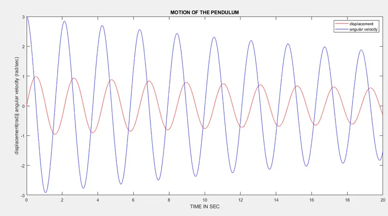
GRAPH 1

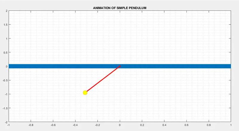
GRAPH 2

animation of the simple pendulum

6. CONCLUSION:

1. The Matlab code that solves the ODE of the simple pendulum with damping has been successfully written.
2. The graphs for angular displacement and angular velocity for each value of time have been plotted.
3. The animation of the pendulum for each and every position is created.

7.REFERENCES:

1. https://skill-lync.com/knowledgebase/understanding-ode45-2
2. https://skill-lync.com/knowledgebase/understanding-anonymous-functions-in-matlab-2