Week 4.1 - Genetic Algorithm

Code about : To optimise the given stalagmite function and find the global maxima of the function .

Introduction to Stalagmite :

Stalagmite structure are formed from the cave floor that poiint upward.Stalagmite function are mathematical functions which represents shapes similar to that of the stalagmite function.Mathematical model that actually helps us to innovate the local minima and maxima.Its is 3D function have local maximas ,global maxima.

Stalagmite function & its Program :

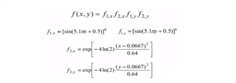
Program For Stalagmite Function :

function Y = stalagmite_fun(input_vector)

x = input_vector(1);
y = input_vector(2);
f1 = (sin(5.1*pi*x+0.5)).^6;
f2 = (sin(5.1*pi*y+0.5)).^6;
f3 = exp((-4*log(2)*((x-0.0667).^2))/0.64);
f4 = exp((-4*log(2))*((y-0.0667).^2)/0.64);
Y =-(f1*f2*f3*f4);
end

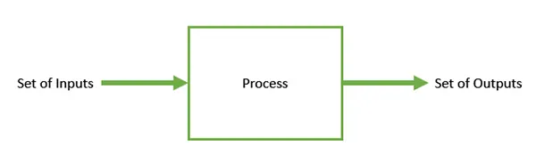
Optimization:- It is a basically area of study that deals with how to minimize or maximize a particular function which

depends upon multiple parameter.

GA (Genetic Algorithm):

GAs are search based alogrithms based on the concepts of natural selection and genetics .GAs area subset of a much larger branch of computation known as Evolutionary computation.GAs were developed by John Holland and his student and colleagues at the university of Michigan most notably David E . Goldberg and has since been tried on Various problems.for getting to know GA also we should know about Failure of gradient based method.

GA Motivation:

This have 'good enough' solution 'fast enough' .In most ofd the real world situations,wwe have a very complex problem called as landscapes which are made of many peaks and valleys which causes such method to fail as they suffer from an inherent tendency of getting stuck at the local optima .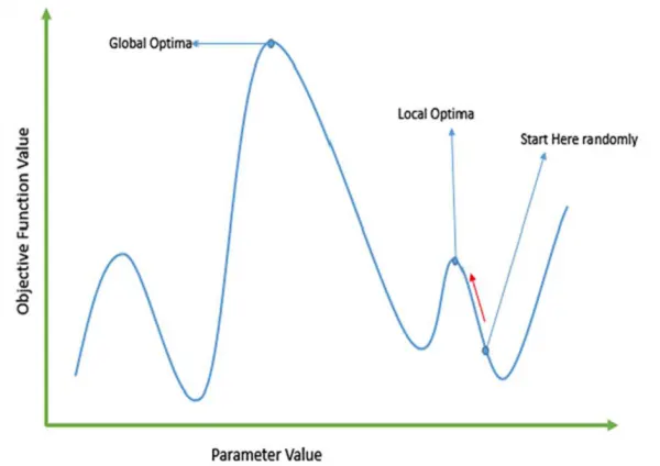

Basic Structure :

It generate random intial population ,selects parents from this population for mating.And then apply crossover andf mutation operators on the parent to generate new offsprings.And finally these off springs replace the existing individual in the population and the process repeats .

Stopping Criteria :

1. Generations : This Stops when the number of generations reaches the values of generation.
2. Time : After Running for an amount of time in seconds its equal to time limit.
3. Fitness : When the value of the fitness function for the best point in the current population is less than or its equal to fitness limit.

Syntax for GA :

x = ga(fun,nvars)

x = ga(fun,nvars,A,b)

x = ga(fun,nvars,A,b,Aeq,beq)

x = ga(fun,nvars,A,b,Aeq,beq,lb,ub)

x = ga(fun,nvars,A,b,[],[],lb,ub,nonlcon,intcon)

x = ga(" ,options)

x = ga (problem)

[x,fval]=ga(_____)

[x,fval,exitflag,output] = ga(___)

[x,fval,exitflag,output,population,scores]=ga(___)

Examples with explanation :-

x = ga(fun,nvars) :- finds a local unconstrained minimum x,to the objective function ,fun.nvars is the dimension (number of design variables) of fun .

[x,fval,exitflag,output,population,scores]=ga(___) :- ga (__)also returns a matrix population whose rows are the final population and a vvector scores,the scores of the final population.

Program :-

clear all
close all 
clc 
x = linspace(0,0.6,150);
y = linspace(0,0.6,150);
num_cases = 70
%Creating a 2 Dimensional Mesh 
[ xx yy ] = meshgrid(x,y);

%Evaluating the stalagmite function
for i=1:length (xx)
    for j=1:length (yy)
    input_vector(1) = xx (i,j);
    input_vector(2) = yy (i,j);
    f(i,j) = stalagmite(input_vector);
    end
end
% f = ga_stalagmite_fun(x,y);

tic
%study 1-statistical behaviour
for i=1:num_cases
    [input,fopt(i)] = ga(@stalagmite_fun,2);
    xopt(i)=input_vector(1);
    yopt(i)=input_vector(2);
end

study1_time = toc
figure(1)
subplot(2,1,1)
hold on
surfc(x,y,f)
shading interp
plot3(xopt,yopt,fopt,'marker','o','markersize',5,'markerfacecolor','r')
title('unbounded inputs')
subplot(2,1,2)
plot(fopt)
xlabel ('interations')
ylabel ('function minimum')

tic 
% study 2 - statistical behaviour - with upper and lowerbounds
for i = 1 : num_cases
    [input,fopt(i)] = ga(@stalagmite,2,[],[],[],[],[0;0],[1;1]);
    xopt(i) = input(1);
    yopt(i) = input(2);
end
study2_time = toc

figure (2)
subplot (2,1,1)
hold on 
surfc (x,y,f)
shading interp 
plot3(xopt,yopt,fopt,'marker','o','markersize',5,'markerfacecolor','r')
title('bounded inputs')
subplot(2,1,2)
plot(fopt)
xlabel ('interations')
ylabel ('function minimum')

% stage 3 increasing GA iterations

options = optimoptions ('ga');
options = optimoptions (options,'PopulationSize',100);
tic
for i = 1 : num_cases
    [input,fopt(i)] = ga(@stalagmite,2,[],[],[],[],[0;0],[1;1],[],[],options);
    xopt(i) = input(1);
    yopt(i) = input(2);
end
study3_time = toc

figure (3)
subplot (2,1,1)
hold on 
surfc (x,y,f)
shading interp 
plot3(xopt,yopt,fopt,'marker','o','markersize',5,'markerfacecolor','r')
title('bounded inputs with increased population')
subplot(2,1,2)
plot(fopt)
xlabel ('interations')
ylabel ('function minimum')

% stage 4 

options = optimoptions ('ga');
options = optimoptions (options,'PopulationSize',300);
tic
for i = 1 : num_cases
    [input,fopt(i)] = ga(@stalagmite,2,[],[],[],[],[0;0],[0.5;0.5],[],[],options);
    xopt(i) = input(1);
    yopt(i) = input(2);
end
study4_time = toc

figure (4)
subplot (2,1,1)
hold on 
surfc (x,y,f)
shading interp 
plot3(xopt,yopt,fopt,'marker','o','markersize',5,'markerfacecolor','r')
title('bounded inputs with increased  extra population')
subplot(2,1,2)
plot(fopt)
xlabel ('interations')
ylabel ('function minimum')

Result :-

study_time_1 : 6.9271

study_time_2 : 7.0459

study_time_3 : 11.6957

study_time_4 : 28.3409

Valuess of x&y for maximum value of function :-

input =

0.0668 0.0668