Challenge

Week 4.1 - Genetic Algorithm

GGowtham N5 May 2022

MATLAB

AIM

To write a code in to optimise the stalagmite function and find the global maxima of the function.

OBJECTIVE

To understand the concept of genetic algorithm

To plot the graph for F maxmum vs iterations

THEORY

Genetic algorithm:genetic algorithm (GA) is a method for solving both constrained and unconstrained optimization problems based on a natural selection process that mimics biological evolution.

Genetic algorithms are commonly used to generate high-quality solutions to optimization and search problems by relying on biologically inspired operators such as mutation, crossover and selection.

Fitness function and Crossover techniques are the two main features of the Genetic Algorithm.

Fitness function:a function which takes a candidate solution to the problem as input and produces as output how “fit” or how “good” the solution is with respect to the problem in.

Crossover techniques:a genetic operator used to vary the programming of a chromosome or chromosomes from one generation to the next.

PROGRAM FOR FUNCTION

function f = stalagmite(input_vector)
x = input_vector(1);
y = input_vector(2);

f1x = (sin(((5.1*pi).*x)+0.5)).^6;

f1y = (sin(((5.1*pi).*y)+0.5)).^6;

f2x = exp((((x-0.0667).^2).*(-4*log(2)))./0.64);

f2y = exp((((y-0.0667).^2).*(-4*log(2)))./0.64);


f = -f1x*f1y*f2x*f2y;
end

FUNCTION CODE EXPLANATION

The stalagmite function is defined and it is later used in main ga program

function command is used to call the function followed by file name(stalagmite is function name) and the input inside the brackets(input_vector).

now we define the x and y followed by set of equations which is as follows

f1x=(sin((5.1*pi).x)+0.5)).^0.6

f1y=(sin((5.1*pi).y)+0.5)).^0.6

f2x=exp((((x-0.667).^2).*(-4log(2)))./0.64)

f2y=exp((((y-0.667).^2).*(-4log(2)))./0.64)

and for the final output multiply all the equation using f as variable -f1x*f1y*f2x*f2y*

end command is used the close the function

MAIN PROGRAM CODE

close all
clear all
clc

x=linspace(0,0.6,150);
y=linspace(0,0.6,150);
num_cases=50
%f=stalagmite(x,y)
[xx,yy]=meshgrid(x,y)
for i = 1: length(xx)
    for j =1:length(yy)
        inputs(1)=xx(i,j);
        inputs(2)=yy(i,j);
        f(i,j)=stalagmite(inputs);
    end
end                    

%study 1 statistical behavior 
for i=1:num_cases
    [inputs,fopt(i)]=ga(@stalagmite,10);
    xopt(i)=inputs(1);
    yopt(i)=inputs(2);
end
study1_time=tic;
figure(1)
subplot(2,1,1)

surfc(x,y,-f)
shading interp
hold on

plot3(xopt,yopt,-fopt,'marker','o','markersize',5,'markerfacecolor','r')
title('unbounded inputs')
subplot(2,1,2)
plot(-fopt)
xlabel('iterations')
ylabel('function')

tic
%study2 statistical behavior with upper bound and lower bound
for i=1:num_cases
    [inputs,fopt(i)]=ga(@stalagmite,2,[],[],[],[],[0;0],[1;1]);
    xopt(i)=inputs(1);
    yopt(i)=inputs(2);
end
study2_time=tic;
figure(2)
subplot(2,1,1)

surfc(x,y,-f)
shading interp
hold on
plot3(xopt,yopt,-fopt,'marker','o','markersize',5,'markerfacecolor','r')
title('bounded inputs')
subplot(2,1,2)
plot(-fopt)
xlabel('iterations')
ylabel('function')

%study 3 | statistical behavior 
options=optimoptions('ga');
options=optimoptions(options,'populationsize',450);
for i=1:num_cases
    [inputs,fopt(i)]=ga(@stalagmite,2,[],[],[],[],[0,0],[0.6,0.6],[],options);
    xopt(i)=inputs(1);
    yopt(i)=inputs(2);
end
study3_time=tic;
figure(3)
subplot(2,1,1)
surfc(x,y,-f)
shading interp
hold on
plot3(xopt,yopt,-fopt,'marker','o','markersize',5,'markerfacecolor','r')
title('unbounded inputs with modified population size')
subplot(2,1,2)
plot(-fopt)
xlabel('iterations')
ylabel('function')

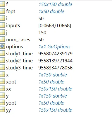
WORKSPACE

SYNTAX OF ga and explanation

x = ga(fun, nvars, A, b, Aeq, beq, lb, ub, nonlcon, options)

1. x is the local minima point.

2. fun is the function to be called. (In our case,its the stalagmite function)

3. nvars indicates the no of variables used.

4. A and b are used to indicate any kind

inequalities that exist in the function.

5. Aeq and Beq also denotes the inequalities.

6. lb= lower bound.

7. ub= upper bound.

8. nonicon gives a two vectors representing inequalities and equalities.

9. options is used to perform additional operations like increasing population size. This is done with the help of "optimoptions".

MAIN PROGRAM CODE EXPLANATION

*The satalagmite function is defined separately. This function is later called into the main GA program.

*Now we define the x and y inputs using linspace command.

* Then the input vectors are transformed into array [xx,yy], so that it can be used to evaluate functions of two variables and plot three-dimensional mesh/surface plots.

* Now the values in the different matrixs created can be put as an input into the function that we have created, by calling it.By this we can get the value of the stalagmite function at various values of x and y.

*Now since we have got the value of the function at various values, we now need to calculate the maxima value, which can be calculated using the ga command, which is an in-built function in MATLAB.

*Then, the total number of time the ga needs to run is defined using num_cases, and with help of for loop ga is made to run for each iteration and the value is stored in an array.

* GA generally gives the minima value (in built in MATLAB), but we need the maxima hence we can just inverse the stalagmite function by introducing a 'Negative sign' (This inverses the stalagmite curve and the Global maximas can be found, instead minima)stalagmite curve and the Global maximas can be found, instead minima)

* The total study time is calculated using the 'tic' and 'toc' command at the start and end of the ga for loop respectively.

*The results are then plotted using the surfc command and plot command.

*ga is made to run for 3 iterations, with each iteration having bounded inputs, unbounded inputs and increasing population size.

OUTPUT FOR 1st STUDY

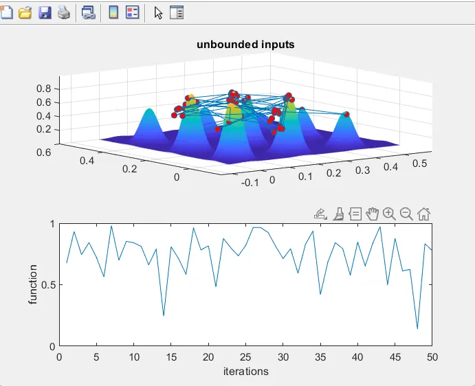
in this case it can be seen that since the inputs are boundaries ga algorithm has mapped

local maxima points outside our stalagmite function .also we cannot infer a particular value for global maxima from the above garph

OUTPUT FOR 2nd STUDY

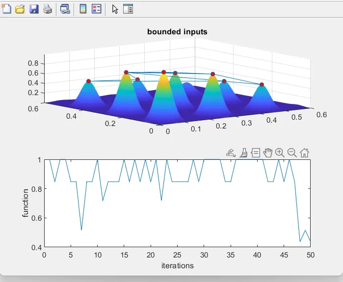
the above graph is more clear and optimized compared to the 1st graph the bounds here were defined and we could get only the values within the range .we are now more clear on the range within our maxima lies

OUTPUT FOR 3rd STUDY

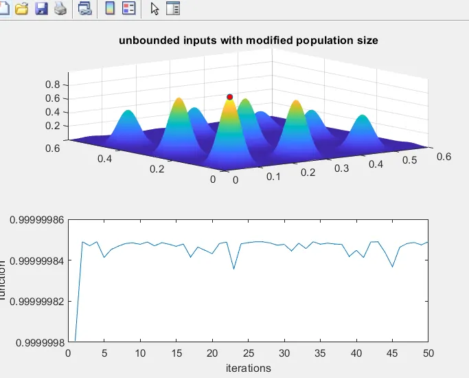
in this case we are getting the optimised value of global maxima with accurate range since we increased the number of iterations and population size

the study time is high compared when compared to the other two.

CONCLUSION

GA gives more accurate results in case of particular search space for ga,the ga doesnt run the inside the search space .only in cases of bounded inputs we can get interferable results

Week 4.1 - Genetic Algorithm

Ship work like this
in your own course.

Talk to a career counsellor

Ship work like thisin your own course.

Talk to a career counsellor

Ship work like this
in your own course.