Week 4.1 - Genetic Algorithm
GENETIC ALGORITHM
Genetic algorithm is an optimization method that can be used to find the global minima and maxima. Genetic algorithm (henceforth GA), is a robust optimization method that has proved to find the best solution in complex or multinodal problems where generic or predefined standard optimization techniques fail.
GA is based on Darwinian theory of evolution that is commonly stated as ‘Survival of the fittest’. What it means in practicality or application is not far from the statement. In nature or in any environment, the fittest species survives the best. For example, during ice age, woolly mammoths or other animals that can store fats and heat in their body survived better and those which didn’t, did not survive the cold and froze to death. This way their species was carried forward. Now in the example of mammoth itself, we can see that the mammoths that evolved during the rising temperatures, survived with the ability to dissipate heat, while mammoths that didn’t evolve, died due to the inability to dissipate heat, also due to shrinking of land coverage during the period of planet warm up.
Similarly the algorithm selects the best genes or data sets from available data and carries them forward by various means. The GA uses steps or methods which are, Initial population, fitness function, selection, cross over and mutation.
The initial population is essentially the initial dataset that you provide.
Fitness function determines how fit an individual data is. It gives a fitness score to each individual data. The probability that a data will be selected for reproduction is based on its fitness score.
Selection phase corresponds to selecting the best individual data for reproduction of next generation, which will be closer to the solution than the previous/parent generation.
Cross-over is a method of reproduction where the best bits of parental genes are selected and mix matched for better data in he next generation.
Mutation is a process where a portion of genetic code is flipped or changed without taking any genes from other individuals to create new generation/off-springs of better fitness value.
Now after understanding the basic model of genetic algorithm, application of genetic algorithm (or GA here onwards) in programming and solution optimization is the next part.
GA minimizes any given function or mathematical model to give the optimum solution. All the above mentioned parameters like the cross over, mutation and also other parameters like population size, Initial population range and iterations quantity can be controlled to achieve the desired output/ better/accurate output.
Population size refers to the quantity of initial values taken in by the algorithm for testing and creating the next generation. Default population size set by Matlab is 50, so for every variable that you have as an input the population size will be 50 each. Increasing the population size helps increase diversity and increases the chances of better individuals fit for creating next generation.
Initial population range is basically range between which you want the GA to select initial population. This additional condition limits the GA’s initial population only, and does not limit the next generation onwards. Hence second generation onwards GA can go anywhere beyond the initial range mentioned. This parameter helps reduce the possibility of GA identifying any local minima as global minima other than actual global minima. The range value needs to be tested over number of implementations and changing the range every time to get the best range. As it turns out, limiting the range directly over the actual solution or global minima doesn’t necessarily help GA but it rather increases the chances of GA identifying a local minima as global minima.
For example, in this given setup in challenge, the answer to the global minima is x & y co-ordinate at 0.0668 and the fitness value or the optimum value is -0.99999985 or when Matlab rounds it up due to short variable settings, it is -1. So if the population range is set to -1 to -0.9, it works well and reduces the chances of identifying local minima as global minima. This range in terms of accuracy is large, as the difference is 0.1. If the accuracy is tried to be increased by reducing the range to the known range of global optima, down to the decimal power of 6 or 6 decimal spaces, the GA starts identifying local minimas. It is the same even if the accuracy is increased to 2 decimal spaces.
So you can’t control accuracy of solution with initial population range.
The syntax of GA is very simple and easy to implement. Which is as follows:
The shortest form of the GA syntax is:
x = ga(fun,nvars);
In this syntax the GA only takes in the function that is to be minimized and the number of variables the function has. This line of code returns the value x on the left hand side which is supposed to be the location of global minimum.
In a different variant of the same code:
[x,fval] = ga(fun,nvars);
There are two outputs on the left hand side now, where x being the same mentioned as above, the variable fval stores the value of the fitness function of the global minimum.
The longest form of syntax for GA is:
x = ga(fun,nvars,A,b,Aeq,beq,lb,ub,nonlcon,options)
In this code the GA is limited or customized in various ways such as limiting the upper and lower values of the variables in the function, which is the lb and ub variables in the code line above. The A and b, variables are the linear inequality definition, while Aeq and beq are linear equalities definition. If the function is not linear at all, or is non-linear then the constraints required are given as input in the ‘nonlcon’ variable irrespective of them being equalities or inequalities. Last is options, which control the various parameters of the GA, which control the output of the optimization algorithm. Options can be given values such as population size, which is the initial population size that the GA starts with, Initial population range being another as explained above.
Another long syntax variant is:
x = ga(fun,nvars,A,b,[],[],lb,ub,nonlcon,IntCon,options)
In this syntax the GA requires the variables listed in the ‘Intcon’ take only integer variables. When this condition is applied, GA does not take linear or non-linear equalities, it only takes in inequalities.
The left hand side of the code has more syntax as well:
[x,fval,exitflag,output] = ga(___)
and
[x,fval,exitflag,output,population,scores] = ga(___)
The first syntax returns exitflag, an integer identifying the reason the algorithm terminated, and output, a structure that contains output from each generation and other information about the performance of the algorithm. While the second syntax also returns a matrix population, whose rows are the final population, and a vector scores, the scores of the final population.
Now GA being an optimization algorithm, there are ways to test it, the most popular one being, making the algorithm find the global minima of a function which is already known. These functions that are used to test optimization algorithms have many varieties in them. Such as Rastrigin’s Function, Ackley’s Function, Sphere function, Rosenbrock’s Function, Beale Function, Goldstein-Price function, Booth function, bukin function, Levi Function, McCormick function, etc. There are many more functions like them to test optimization algorithms.
In the given assignment, the Stalagmite function was given as a test function to test the GA. Stalagmite function generates (when generated a surface graph in 3D) peaks which resembles Stalagmites (which are found in caves where high mineral deposition is found and water droplets carry those minerals and form peak like structures over a period of time).
The function code for Stalagmite function is as follows:
function [A] = stalagmite(input_vector)
x = input_vector(1);
y = input_vector(2);

f1x = (sin((5.1*pi.*x)+0.5)).^6;
f2x = exp((-4)*log(2).*((x-0.0667).^2)./0.64);

f1y = (sin((5.1*pi.*y)+0.5)).^6;
f2y = exp((-4)*log(2).*((y-0.0667).^2)./0.64);

A = f1x.*f2x.*f1y.*f2y;
end
And the code for running the stalagmite function is as follows:
clear all
close all
clc

%defining our search space
x = linspace(0,0.6,150);
y = linspace(0,0.6,150);

%creating two dimensional mesh
[xx, yy] = meshgrid(x,y);

%evaluating the stalagmite function
for i=1:length(xx)
    for j=1:length(yy)
        input_vector(1)=xx(i,j);
        input_vector(2)=yy(i,j);
        f(i,j)=stalagmite(input_vector);

    end
end

surfc(xx,yy,f)
shading interp
The above function results in the following 3D output:
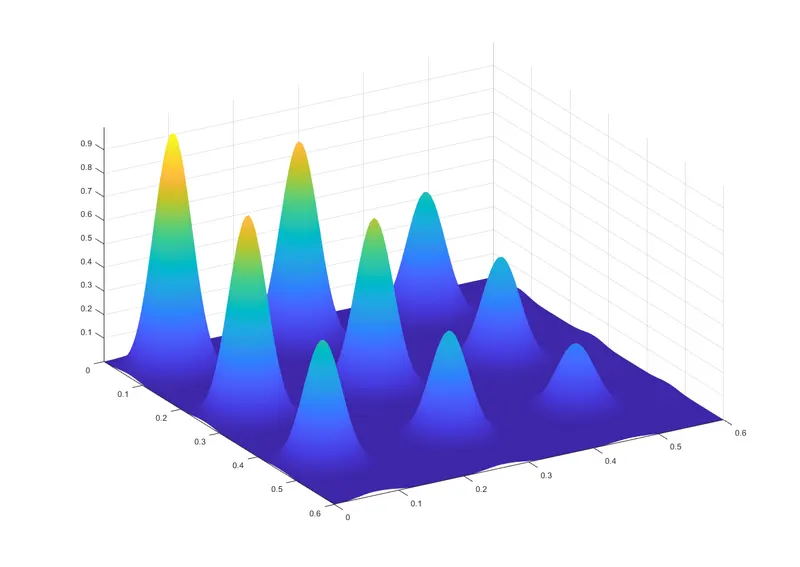
As you can see the function generates various peaks, each having different altitude. But the lowest possible value in this function is Zero, as it is visually evident. When GA is used to optimize this function, Ga will return the lowest value as zero. But as you can see, Zero as a value is present in many spaces and GA will return different location everytime it is executed.
Now in the given assignment, we were asked to identify the location with maximum value or in other words, we were to maximize the function using Ga. To make that possible, a small tweak to the stalagmite function was required, which is shown below:
function [A] = stalagmite(input_vector)
x = input_vector(1);
y = input_vector(2);

f1x = (sin((5.1*pi.*x)+0.5)).^6;
f2x = exp((-4)*log(2).*((x-0.0667).^2)./0.64);

f1y = (sin((5.1*pi.*y)+0.5)).^6;
f2y = exp((-4)*log(2).*((y-0.0667).^2)./0.64);

A = -(f1x.*f2x.*f1y.*f2y);
end
This function will produce a reverse 3D graph of what is shown above, in other words, it will create stalactite graph.
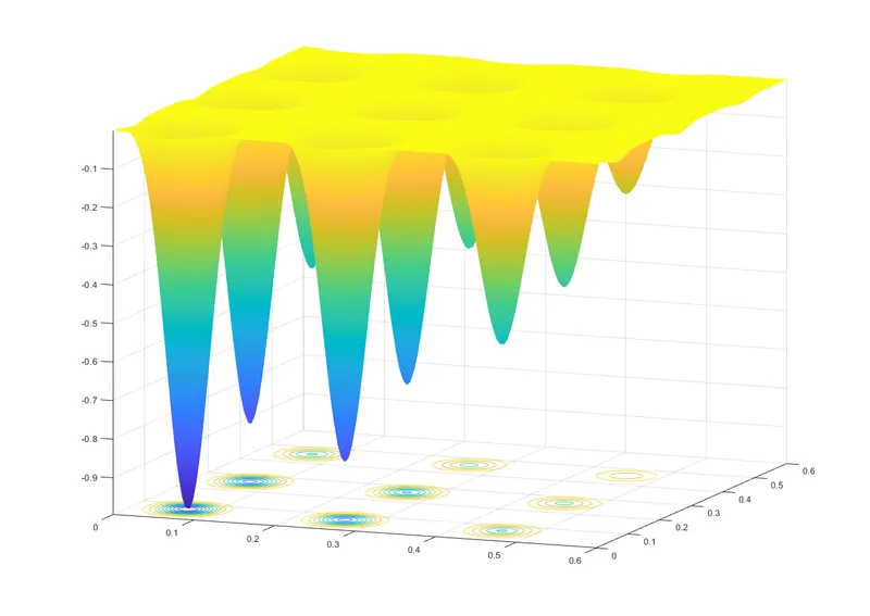
Thus adding the code line (given below) at the end of the main code which uses the stalagmite function uses GA to find the minimum value or it minimizes the function, which is essentially the maximum value possible in the function with the given parameters.
[inputs, fval]= ga(@stalagmite, 2)Thus the code is rewritten as:
clear all
close all
clc

%defining our search space
x = linspace(0,0.6,150);
y = linspace(0,0.6,150);

%creating two dimensional mesh
[xx, yy] = meshgrid(x,y);

%evaluating the stalagmite function
for i=1:length(xx)
    for j=1:length(yy)
        input_vector(1)=xx(i,j);
        input_vector(2)=yy(i,j);
        f(i,j)=stalagmite(input_vector);

    end
end

surfc(xx,yy,f)
shading interp
[inputs, fval]= ga(@stalagmite, 2)
The output to it is:
Optimization terminated: average change in the fitness value less than options.FunctionTolerance.
inputs = 0.0753 0.0939
fval = -0.5266
Here inputs refer to x and y coordinates respectively, while fval refers to the minimum value in the function. But if we see the surface graph, it is clearly visible that the lowest possible value by the stalagmite function is -1 or near -1. That means the GA is providing wrong values. To correct that, 4 steps or types of studies are used. Out of which 3 are explained by the instructor and the 4th or last one being developed by myself.
In all the 4 studies the output of the GA will be compared with visual graph as shown above.
To conduct these studies, we need to run the above mentioned code that calls the stalagmite function. Thus the above code is converted into a function code as below:
function [f] = get_stalagmite(x,y)
a=x;
b=y;

%creating two dimensional mesh
[xx, yy] = meshgrid(a,b);

%evaluating the stalagmite function
for i=1:length(xx)
    for j=1:length(yy)
        input_vector(1)=xx(i,j);
        input_vector(2)=yy(i,j);
        F(i,j)=stalagmite(input_vector);

    end
end
f = F;
end
The First study/step
The first step/study is to increase the number of iterations of GA. Until now, GA was executed only once and hence it would return only one possible value for minimization. Thus to understand the spectrum where GA is detecting the values, we will increase the number of iterations.
The code for that is as follows:
% ga study 1

clear all
close all
clc

x = linspace(0,0.6,150);
y = linspace(0,0.6,150);
num_cases = 50;
f = get_stalagmite(x,y);

tic
%study 1 statistical behaviour
for i=1:num_cases
    [inputs, fopt(i)] = ga(@stalagmite,2);
    xopt(i) = inputs(1);
    yopt(i) = inputs(2);
end

study1 = toc

figure(1)
subplot(2,1,1)
hold on
    surfc(x,y,f)
    shading interp
    plot3(xopt,yopt,fopt,'marker','o','markersize',5,'markerfacecolor', 'r')
	xlabel('x values')
	ylabel('y values')
    title('unbounded inputs')
    subplot(2,1,2)
    plot (fopt)
    xlabel('iterations')
    ylabel('function minimum')
The code has three parts to it and also the next 3 study codes will have same format except minor tweaks. After clearing all previous data, the variables are taken as an input, which are x, y, num_cases and f. Variable f is given value by calling the function ‘get_stalagmite’ which calls the stalagmite function to calculate values. num_cases is used for determining the number of times iteration must be run. The second part is a for loop which runs the GA for number of iterations mentioned in the variables above.
The third part is coded to plot out the 3D surface graphs and all the iterative outputs that the GA produces as well as the their respective minimal value against the number of iterations.
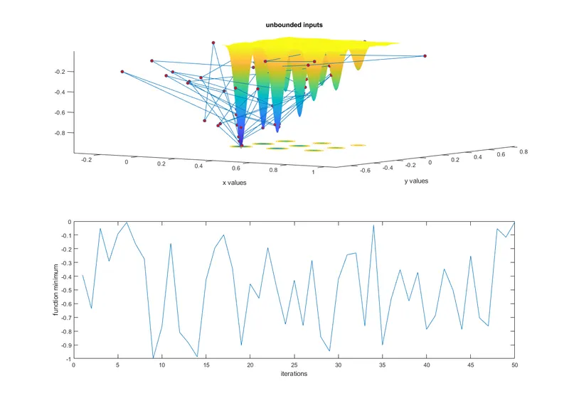
The image above has 2 parts, the first/top part is a surface graph just as same shown above, along with the points detected as the global minimum by the GA. The second part or the bottom part is the value of global minimum detected by the GA versus the iterations.
The top graph clearly helps visualize how out of bounds or random the GA’s detection goes regarding the global minimum. That is because Ga is executed unconstrained. Due to that after the default number of generations or when GA stops making progress in accuracy it terminates with the value having best fitness function. This can be anywhere because its not constrained.
The other part of the reason behind GA detecting values outside the graph is due to its genetic mutation and crossover. In mutation as explained before, a portion of gene of the value is switched, changed, or flipped randomly to create diversity. Due to which any value can be generated, even the ones outside the required region or graph.
To avoid the above difficulties, the GA needs to be constrained. For which the code is tweaked a little in the second study/step.
The second study/step
In the second study/step, the GA will be bounded to upper and lower bounds, which will define the limits of values of GA. This way the GA won’t consider values that are outside the bounds formed during the mutation and crossover. The code for the second study or step is as follows:
% ga study 2 with lower and upper bounds
clear all
close all
clc

x = linspace(0,0.6,150);
y = linspace(0,0.6,150);
num_cases = 50;
f = get_stalagmite(x,y);

tic
for i=1:num_cases
    [inputs, fopt(i)] = ga(@stalagmite,2,[],[],[],[],[0;0],[1;1]);
    xopt(i) = inputs(1);
    yopt(i) = inputs(2);
end

study2 = toc

figure(1)
subplot(2,1,1)
hold on
    surfc(x,y,f)
    shading interp
    plot3(xopt,yopt,fopt,'marker','o','markersize',5,'markerfacecolor', 'r')
    xlabel('x values')
    ylabel('y values')
    title('unbounded inputs')
    subplot(2,1,2)
    plot (fopt)
    xlabel('iterations')
    ylabel('function minimum')
The changes made to this code are in the function details of GA. After the four blank spaces, which are for inputs regarding linear and non linear equalities of the function, the inputs for upper and lower bounds are given, being [0;0] and [1;1] whose syntax is [x1;y1],[x2;y2]. This way the values of x and y wont go outside 0 and 1.
Output to the code above
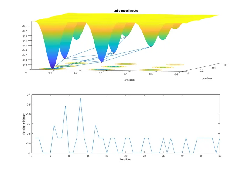
As visible from the graph above, the variation in identification of global minimum by GA has reduced drastically down to 6 points. Yet this is not the absolute solution. Having 6 different global minimums is not a solution. Thus to reduce the variation further down, the third study makes further changes to the code.
The third study/step:
The problem concerning to us can also be solved by increasing the initial population size. The default population size given by matlab for GA is 50 for each variable. Thus the population size is increased using the options command. The code is given below:
% ga study 3
clear all
close all
clc

x = linspace(0,0.6,150);
y = linspace(0,0.6,150);
num_cases = 50;
f = get_stalagmite(x,y);

options = optimoptions('ga');
options = optimoptions(options, 'PopulationSize', 170);

tic
for i=1:num_cases
    [inputs, fopt(i)] = ga(@stalagmite,2,[],[],[],[],[0;0],[1;1],[],[],options);
    xopt(i) = inputs(1);
    yopt(i) = inputs(2);
end

study3 = toc

figure(1)
subplot(2,1,1)
hold on
    surfc(x,y,f)
    shading interp
    plot3(xopt,yopt,fopt,'marker','o','markersize',5,'markerfacecolor', 'r')
    xlabel('x values')
    ylabel('y values')
    title('unbounded inputs')
    subplot(2,1,2)
    plot (fopt)
    xlabel('iterations')
    ylabel('function minimum')
The output to the above code is:
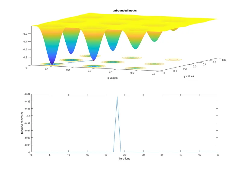
study3 = 8.2653
As visible, the variation is reduced down to two values which rarely goes up to 3 but mostly has only 2 variants, and under very rare circumstances does it show only one, which it should naturally show. But since that is not the case, the code is further modified or refined if said specifically for repeatability.
The fourth study/step:
It was suggested that increasing the number of iterations will solve the problem. But that doesn’t necessarily rule out the probability of GA detecting a local minima.
Increasing the initial population size does changes the chances of GA detecting a local minima, but yet there are occurrences of local minima at least twice or thrice for every 50 iterations. Thus in order to reduce the chances we will set a population range that the GA will begin with. This parameter is explained to start of the document/answer.
Applying that parameter drastically reduced the chances or pretty much made it impossible for GA to detect the local minimas. Initially a wide range was applied, which was then narrowed down to the current value applied in the program as with each change the program was run for 10 times, where at least once the local minima was detected. With each change, the range was narrowed down to the global minima value. Apparently keeping the range anywhere near the global minima with a minimum difference of 0.1 will definitely result in GA detecting global minima, straying further away increased chances of local minima being detected. Also reducing the range gap below 0.1 also backfired, where the GA started detecting more local minimas than the previous step.
One minute change was to increase the population size to 300 or as large as possible, as it introduces the variety and increases the chances of GA detecting only the global minima.
After increasing repeatability, it was observed that GA did detect the global minima, but the value at that point varied with each iteration, but at the scale of 1e-8 or after the 6th or 7th decimal space. The value being in such large decimals can be rounded up to 4 decimal spaces and a common answer will be derived. But for applications requiring higher accuracy, the value can be processed which differ at higher decimal spaces. To do that a filter is be applied which creates 2 sets of value, one at 4 decimal space accuracy and another at 7 decimal space accuracy. And the values were plotted and compared to demonstrate the difference accuracy makes while plotting or calculations.
The code for the fourth study/step is as follows:
% ga study 4

clear all
close all
clc

x = linspace(0,0.6,150);
y = linspace(0,0.6,150);
num_cases = 120;
f = get_stalagmite(x,y);

%options.CrossoverFraction = 1; %matlab default 0.8 applying this command
%makes no change yet it can be still applied if required.
options = optimoptions('ga', 'PopulationSize', 300,'InitialPopulationRange',[-1;-0.9]);

tic
xopt = zeros(1,num_cases);
yopt = zeros(1,num_cases);
fopt = zeros(1,num_cases);

for i=1:num_cases
    [inputs, fopt(i)] = ga(@stalagmite,2,[],[],[],[],[0;0],[0.6;0.6],[],[],options);
    xopt(i) = inputs(1);
    yopt(i) = inputs(2);
end

study3 = toc

figure(1)
    subplot(3,2,[1,2])
hold on
    surfc(x,y,f)
    shading interp
    plot3(xopt,yopt,fopt,'marker','o','markersize',5,'markerfacecolor', 'r')
    xlabel('x values')
    ylabel('y values')
    title('inputs')

    %plotting raw fopt value
    subplot(3,2,[3,4])
    plot (fopt)
    xlabel('iterations')
    ylabel('function minimum')
    title ('raw output')

    %plotting fopt value procesed/rounded upto 7 decimal places
    F = round(fopt.*10000000)./10000000;
    subplot(3,2,5)
    plot (F)
    xlim([0 120])
    ylim([-1 -0.9999995])
    xlabel('iterations')
    ylabel('function minimum')
    title ('processed output with accuracy 1x10e-7')

    %plotting fopt value procesed/rounded upto 4 decimal places
    H = round(fopt.*10000)./10000;
    subplot(3,2,6)
    plot (H)
    xlim([0 120])
    ylim([-1.0000001 -0.9999998])
    xlabel('iterations')
    ylabel('function minimum')
    title ('processed output with accuracy 1x10e-4')
and the corresponding output is as follows:
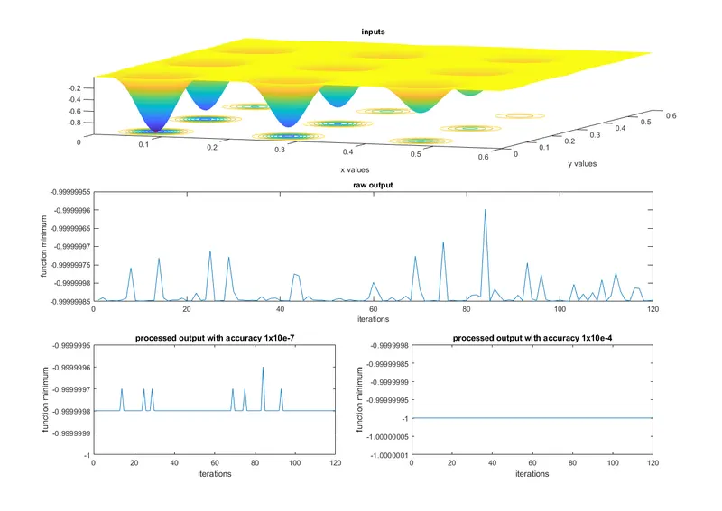
First and foremost, the GA detects only one location as mentioned above. Which is a great development in terms of repeatability. Second, the value at that location varies at a long length of decimals, which creates concerns for problems requiring high accuracy. As you can see, the value ranges from -0.99999955 to -0.99999985. Although a small number and even smaller difference, applications like C.F.D. require accuracy upto 9th decimal spaces, for whom this is a bad thing. Thus further development needs to be done to increase accuracy. Although with current knowledge and understanding, this is the best solution that can be created.
Further more applications which do not require that level of accuracy but want to take the values directly from the variable, can apply rounding filters as shown above. This helps us as well to understand the variation in values. The 3rd plot has 7 decimal spaces accuracy and 4th plot has 4 decimal spaces accuracy. As you can see the major difference here.
As the value is not -1 but near -1, the higher accuracy filter shows that the value is essentially -0.9999998 and not -1. But when lower accuracy filter is applied, the rounding off causes the value to be -1 and not -0.9999998, which is a considerable difference.
References:
1] https://www.mathworks.com/help/matlab/matlab_prog/display-format-for-numeric-values.html
2] https://www.mathworks.com/help/gads/vary-mutation-and-crossover.html
3] https://www.mathworks.com/help/symbolic/digits.html
4] https://www.mathworks.com/matlabcentral/answers/129689-finding-repetition-numbers-in-array
5] https://stackoverflow.com/questions/31215003/genetic-algorithm-selection-method-stuck-at-local-minimum-after-few-generations
6] https://www.researchgate.net/post/When-we-use-Genetic-Algorithm-how-we-know-the-solution-has-reached-the-global-minima
7] https://link.springer.com/article/10.1007/s11042-020-10139-6
8] https://towardsdatascience.com/introduction-to-genetic-algorithms-including-example-code-e396e98d8bf3
9] https://www.mathworks.com/help/releases/R2021a/gads/genetic-algorithm-options.html#f17822
10] https://en.wikipedia.org/wiki/Test_functions_for_optimization
11] https://www.mathworks.com/help/matlab/ref/maxnumcompthreads.html
12] https://www.mathworks.com/help/releases/R2021a/matlab/matlab_prog/preallocating-arrays.html
13] https://www.mathworks.com/help/releases/R2021a/gads/options-and-outputs.html?s_tid=doc_srchtitle
14] https://www.mathworks.com/help/releases/R2021a/gads/ga.html?s_tid=doc_srchtitle#d123e39116
15] https://www.mathworks.com/help/releases/R2021a/matlab/ref/subplot.html
16] https://www.mathworks.com/help/matlab/creating_plots/change-axis-limits-of-graph.html
17] https://www.mathworks.com/matlabcentral/answers/79928-reduce-precision-of-a-number