Week 4.1 - Genetic Algorithm
Genetic Algorithm
The genetic algorithm is a method for solving both constrained and unconstrained optimization problems that is based on natural selection, the process that drives biological evolution. The genetic algorithm repeatedly modifies a population of individual solutions. At each step, the genetic algorithm selects individuals from the current population to be parents and uses them to produce the children for the next generation. Over successive generations, the population "evolves" toward an optimal solution. You can apply the genetic algorithm to solve a variety of optimization problems that are not well suited for standard optimization algorithms, including problems in which the objective function is discontinuous, nondifferentiable, stochastic, or highly nonlinear. The genetic algorithm can address problems of mixed integer programming, where some components are restricted to be integer-valued.
This flow chart outlines the main algorithmic steps. For details, see How the Genetic Algorithm Work

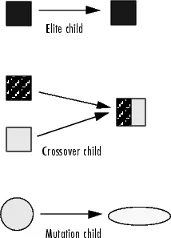
The genetic algorithm uses three main types of rules at each step to create the next generation from the current population:
-
Selection rules select the individuals, called parents, that contribute to the population at the next generation. The selection is generally stochastic, and can depend on the individuals' scores.
-
Crossover rules combine two parents to form children for the next generation.
-
Mutation rules apply random changes to individual parents to form children.
Input Functions
Main Program
clear all
close all
clc

% Determining Search Space
x = linspace(0,0.6,150); % Values for X
y = linspace(0,0.6,150); % Values for Y
[xx,yy] = meshgrid(x,y); %Creating 2 D grid with x and y values

%calling the Stalagmite Function
for i = 1:length(xx)
    for j = 1:length(yy)
        input_vector(1) = xx(i,j);
        input_vector(2)= yy(i,j);
        F(i,j) = stalagmite(input_vector);
    end
end

%Iteration Number 1
num_cases_1 = 50; % Number of iterations
tic % Starting the time count

for i = 1:num_cases_1
    [inputs_1,F_optimum_1(i)] = ga(@stalagmite,2);
    x_optimum(i) = inputs_1(1);
    y_optimum(i) = inputs_1(2);
    optimum_function_1(i) = -F_optimum_1(i); % This gives us the maxima value
end

study_time_1 = toc; % Stopping the time count

figure(1)
subplot(2,1,1)
hold on
surfc(xx,yy,-F)
shading interp % To creat smooth curve surface
plot3(x_optimum,y_optimum,optimum_function_1,'Marker','o','MarkerFaceColor','r')
title('Unbounded Data')
subplot(2,1,2)
plot(optimum_function_1)
xlabel('Number of Iterations')
ylabel('F Maximum')


%Iteration Number 2
num_cases_2 = 100; % Number of iterations
tic % Starting the time count

for i = 1:num_cases_2
    % Setting upper and lower boundary
    [inputs_2,F_optimum_2(i)] = ga(@stalagmite,2,[],[],[],[],[0,0],[0.6,0.6]);
    x_optimum(i) = inputs_2(1);
    y_optimum(i) = inputs_2(2);
    optimum_function_2(i) = -F_optimum_2(i); % This gives us the maxima value
end

study_time_2 = toc; % Stopping the time count

figure(2)
subplot(2,1,1)
hold on
surfc(xx,yy,-F)
shading interp % To creat smooth curve surface
plot3(x_optimum,y_optimum,optimum_function_2,'Marker','o','MarkerFaceColor','r')
title('Bounded Data')
subplot(2,1,2)
plot(optimum_function_2)
xlabel('Number of Iterations')
ylabel('F Maximum')

%Iteration Number 3
num_cases_3 = 150; % Number of iterations
options = optimoptions('ga');
options = optimoptions(options,'PopulationSize',450);
tic % Starting the time count

for i = 1:num_cases_3
    % Setting upper and lower boundary
    % We use 'options' to define size of the population
    [inputs_3,F_optimum_3(i)] = ga(@stalagmite,2,[],[],[],[],[0,0],[0.6,0.6],[],options);
    x_optimum(i) = inputs_3(1);
    y_optimum(i) = inputs_3(2);
    optimum_function_3(i) = -F_optimum_3(i); % This gives us the maxima value
end

study_time_3 = toc; % Stopping the time count

figure(3)
subplot(2,1,1)
hold on
surfc(xx,yy,-F)
shading interp % To creat smooth curve surface
plot3(x_optimum,y_optimum,optimum_function_3,'Marker','o','MarkerFaceColor','r')
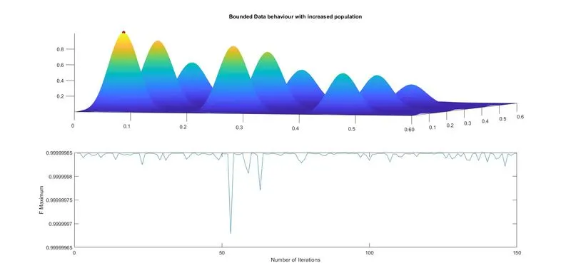
title('Bounded Data behaviour with increased population')
subplot(2,1,2)
plot(optimum_function_3)
xlabel('Number of Iterations')
ylabel('F Maximum')

% Global Maxima of every Iterations is the Maximum value in the
% corresponding 'F_optimum' array
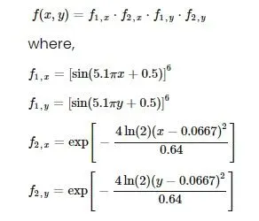
The Stalagmite function Code
% Stalagmite Function that will be called in the maain function.
function [F] = stalagmite(input_vector)

x = input_vector(1);
y = input_vector(2);

F1 = (sin(5.1*pi*x + 0.5)).^6;
F2 = (sin(5.1*pi*y + 0.5)).^6;
F3 = exp((-4*log(2)*(x-0.0667).^2)/(0.64));
F4 = exp((-4*log(2)*(y-0.0667).^2)/(0.64));
F = -F1*F2*F3*F4;
end
Step By Step Explanations Of The Code.
Step 1-Clear all, close all, clc - to clear all the text form workspace,command window and to close all plots.
Step 2-We use 'linspace' command to define array of 150 equaly spaced numbers between 0 and 0.6 and is stored in the vaiables x and y.
Step 3-Now we creat a 2D mesh using 'meshgrid' command with x and y as inputs.
Step 4-Then we use 'for loop' to solve the 'stalagmite' function for every element in the 2D grid.
Step 5-Now we start the 1st iteration.
Step 6-For the 1st iteration number of casses denoted by 'num_cases_1' is 50 and at the start of the iteration we start the time count using command 'tic' to measure the time taken for the iterration.
Step 7-Then a for loop is used which iterate from 1 to number of element in 'num_cases_1'.
Step 8-Then we enter the 'ga' code in MATLAB which has the format '[inputs_1,F_optimum_1] = ga(fun,nvars). Here 'inputs' represent the values of parameter x and y for which the function has least value.
Step 9-The 'fun' and 'nvars' demots the values of parameter x and y for wchich the function has the least values and the number of variables respectively.
Step 10-Now we store the x and y coordinates of the minimum values of the fuction in variables 'x_optimum' and y_optimum' for all 50 iterations.
Step 11-Now we define the varable 'optimum_function' which will be the inverse of the minimum values, therefor 'optimum_function' will be the maxima values.
Step 12-Now we use the command 'toc' to stop the time count and store the time taken for the 1st iteration in the variable 'study_time_1'.
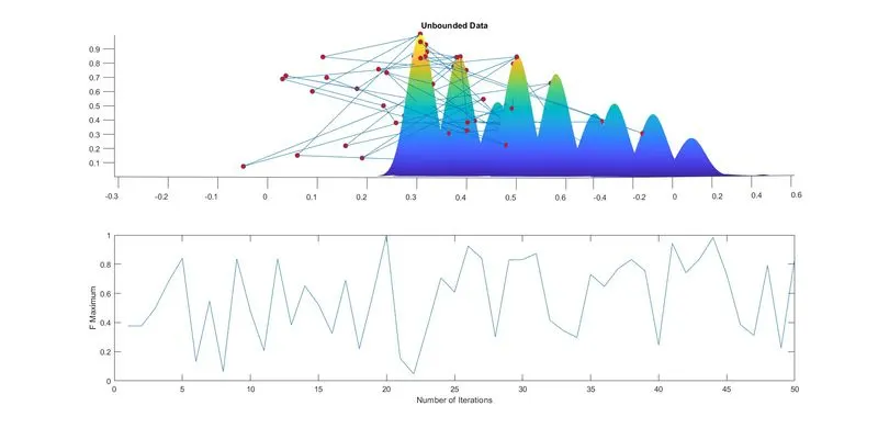
Step 13-Now we plot the figure for the 'unbounded data' by opening a new figure window and using 'subplot' command we can divide the current figure into an m-by-n grid and creates axes in the position specified by p.
Step 14-The 'surfc' command is used to plot contour with 'xx' and 'yy' values and 'optimum_function_1' since we need to represent the maxima of the function.
Step 15-We use 'shading interp' command to smoothen the function plot and to remove grid lines.
Step 16-Then we plot the 'optimum_function_1' on the same figure in the second row.
Step 17-Then we mention the 'xlabel' ,'ylabel' and the 'title'.
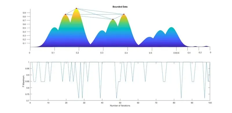
Step 18-Now we do the same procedure for 2nd iteration with 'num_case_2 = 100' (100 iterations) and has upper and lower limits (bounded).
Step 19-We use the 'ga' command with format '[inputs_2,F_optimum_2] = ga(fun,nvars,A,B,Aeq,Beq,lb,ub)'.
Step 20-A, B, Aeq, Beq are linear inequality constraints since all these are none we denot it as '[]'. 'lb' and 'ub' denots lower boundary and upper boundary.
Step 21-Now we plot the 'bounded data' similar to 'unbounded data' by opening another figure window.
Step 22-Now for the third iteration we use the same procedure with 'num_cases_3 = 150' (150 iterations) which has upper and lower bounds and also with increaed population size.
Step 23-Here we use the 'ga' command with format '[inputs_3,F_optimum_3] = ga(fun,nvars,A,B,Aeq,Beq,lb,ub,nonlcon or intcon,options)'.
Step 24-The 'intcon' and 'nonlcon' are integer variables and nonlinear constraints, since both has none values it is denoted as '[]'. Options denotes optimization options.
Step 25-This 'ga' is also bounded but with increase in population size, thus accuracy will be obtained.
step 26-After each iteration the time count is calculated.
Step 27-Now we plot the 'bounded data with incresed population' similar to the previous plots by opening another figure window.
Step 28-Now Global Maxima of every Iterations is the Maximum value in the corresponding 'F_optimum' array.
Step By Step Explanations Of The Stalagmite function Code.
Step 29-We define the function and mention its inputs.
Step 30-We have the equations for a stalagmite function. These equations are written and iputs are assigned.
Step 31-At last we compute the 'F' according to the input vectors.
Results
Plot -1 Unbounded Data
Plot - 2 Bounded Data
Plot - 3 Bounded data with increased population
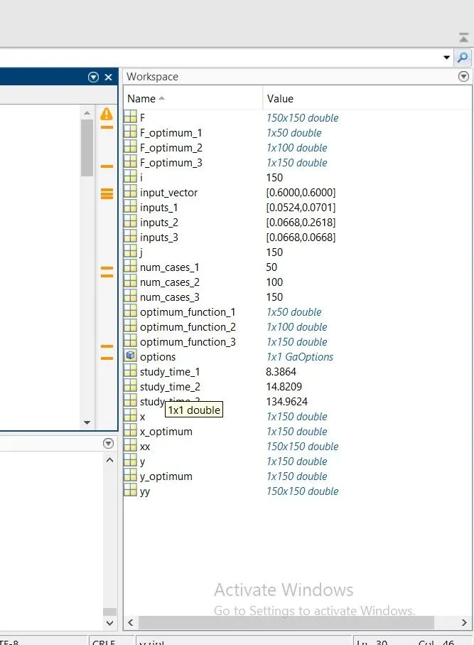
Workspace Data
Syntax for 'ga' in MATLAB
F_min - Local min point.
@function - Calling stalagmite function.
nvars - Number of variables.
A, B, Aeq & Beq - Linear inequality constraints.
lb & ub - Lower and Upper boundary.
nonlcon - Nonlinear constraints.
intcon - Integer variables.
options - Used to perform increase in population calculation.
Errors while programming.
Error 1 - A typo error 'Y = linspace(0,0.6,150)' was typed instead of 'y = linspace(0,0.6,150)'
Solution - Change 'Y = linspace(0,0.6,150)' to 'y = linspace(0,0.6,150)'.
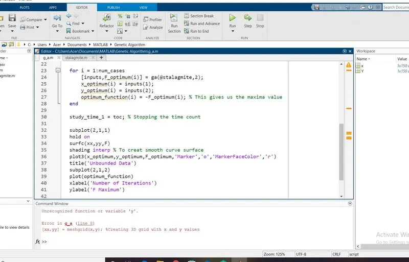
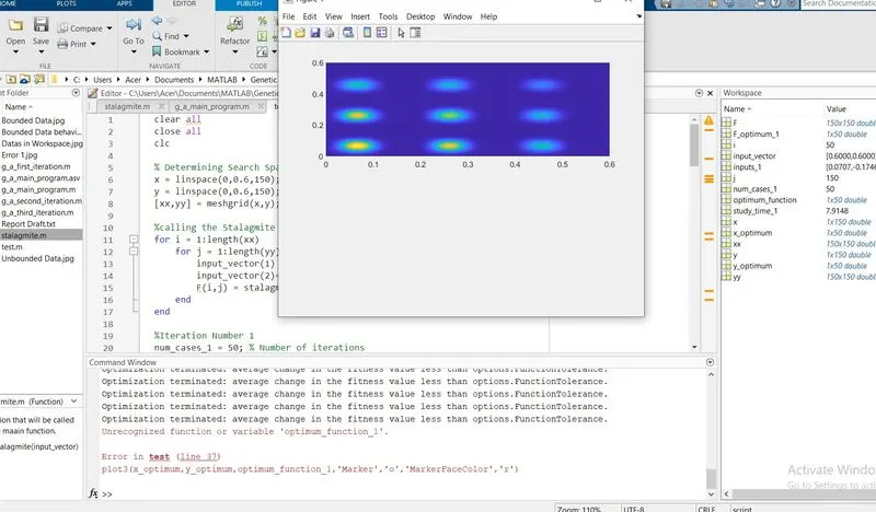
Error 2 - In line 27 'optimum_function' was typed instead of 'optimum_function_1'.
Solution - Change 'optimum_function' to 'optimum_function_1'.
Reference
- https://in.mathworks.com/help/gads/how-the-genetic-algorithm-works.html
- https://in.mathworks.com/help/gads/ga.html
- https://en.wikipedia.org/wiki/Genetic_algorithm
- https://www.geeksforgeeks.org/genetic-algorithms/
- https://towardsdatascience.com/introduction-to-genetic-algorithms-including-example-code-e396e98d8bf3