Week 4.1 - Genetic Algorithm
Aim:1.To optimize the staglamite function and global maxima of function using matlab.
2.And also explain the syntax of genetic algorithm.
Theory:
1.Firstly we define genetic algorithm
Genetic algorithm:It is a method for solving both constrained and unconstrained optimization problem that is based on natural selection,the process that drives biological evolution.The genetic algorithm repeatedly modifies a population of individual solution.At each step, the genetic algorithm selects individual from the current population to be parents and uses them to produce the children for the next generation.Over successive generations,the population evolves toward and optimal solution.Genetic algorithm is apply to solve discontinuous,nondifferential,highly non linear function.
The flow chart outlines the main algorithm steps:
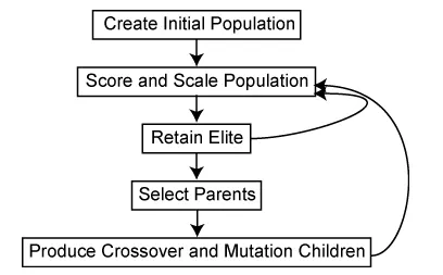
Genetic algorith uses three main types of rules at each step to create next generation from current population:
1.SELECTION
2.CROSSOVER
3.MUTATION
2.What is STAGLAMITE function and syntax
A staglamite function generally refers to the function with which we are generating values over a staglamite kind of surface for finding out the local and global maxima and minima of that particular given function.
Syntax for staglamite function
x=ga(fun,nvars)
x = ga(fun,nvars,A,b)
x = ga(fun,nvars,A,b,Aeq,beq)
x=ga(fun,nvars,A,b,Aeq,beq,lb,ub)
x=ga(fun,nvars,A,b,Aeq,beq,lb,ub,nonlcon)
x=ga(fun,nvars,A,b,Aeq,beq,lb,ub,nonlcon,options)
x=ga(fun,nvars,A,b[],[],lb,ub,nonlcon,Intcon)
x=ga(fun,nvars,A,b[],[],lb,ub,nonlcon,Intcon,options)
x=ga(problem)
[x,fval]=ga(_)
[x,fval,exitflag,output]=ga(_)
[x,fval,exitflag,output,population,scores]=ga(_)
Description of syntax
x=ga(fun,nvars) finds a local unconstrained minimum, x, to the objective function, fun,nvars is the dimension (number of design variables) of fun.
x = ga(fun,nvars,A,b) finds a local minimum x to fun , subject to the linear inequalities A*x ≤ b . ga evaluates the matrix product A*x
as if x is transposed ( A*x' ).
x = ga(fun,nvars,A,b,Aeq,beq) finds a local minimum x to fun , subject to the linear equalities Aeq*x = beq and A*x ≤ b . (Set A=[]
and b=[] if no linear inequalities exist.) ga evaluates the matrix product Aeq*x as if x is transposed ( Aeq*x' ).
x=ga(fun,nvars,A,b,Aeq,beq,lb,ub) defines a set of lower and upper bounds on the design variables, x , so that a solution is found in the
range lb ≤ x ≤ ub . (Set Aeq=[] and beq=[] if no linear equalities exist.)
x=ga(fun,nvars,A,b,Aeq,beq,lb,ub,nonlcon) subjects the minimization to the constraints defined in nonlcon . The function nonlcon
accepts x and returns vectors C and Ceq , representing the nonlinear inequalities and equalities respectively. ga minimizes the fun such
that C(x) ≤ 0 and Ceq(x) = 0 . (Set lb=[] and ub=[] if no bounds exist.)
x=ga(fun,nvars,A,b,Aeq,beq,lb,ub,nonlcon,options)minimizes with the default optimization parameters replaced by values in options .
(Set nonlcon=[] if no nonlinear constraints exist.) Create options using optimoptions .
x=ga(fun,nvars,A,b[],[],lb,ub,nonlcon,Intcon) or x = ga(fun,nvars,A,b,[],[],lb,ub,nonlcon,IntCon,options) requires that the
variables listed in IntCon take integer values.
x = ga(problem) finds the minimum for problem , a structure described in problem .
[x,fval]=ga(_), for any previous input arguments, also returns fval , the value of the fitness function at x .
[x,fval,exitflag,output]=ga(_) also returns exitflag , an integer identifying the reason the algorithm terminated, and output , a
structure that contains output from each generation and other information about the performance of the algorithm.
[x,fval,exitflag,output,population,scores]=ga(_) also returns a matrix population , whose rows are the final population, and a
vector scores , the scores of the final population.
1.STAGLAMITE FUNCTION CODE
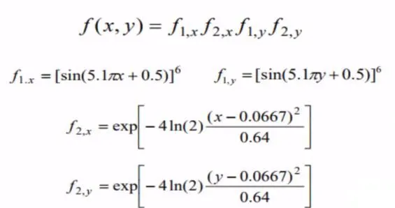
The above eqn used to write stagalmite function.
code:
function A = stagalmite(input_vector)
x=input_vector(1);
y=input_vector(2);
f1=(sin(5.1*pi*x+0.5)).^6;
f2=exp((-4*log(2)*((x-0.0667).^2))/0.64);
f3=(sin(5.1*pi*y+0.5)).^6;
f4=exp((-4*log(2))*((y-0.0667).^2)/0.64);
A =-(f1*f2*f3*f4);
end
Program explanation:

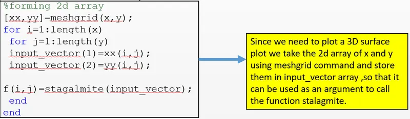
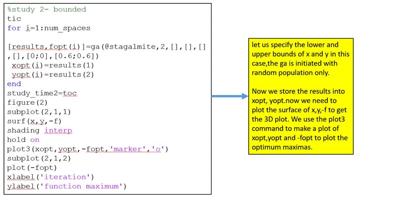
STUDY 1
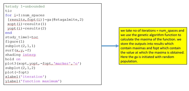
STUDY 2
FINAL PROGRAM
close all
clear all
clc
%input
x=linspace(0,0.8,150);
y=linspace(0,0.8,150);
num_spaces=80;
%forming 2d array
[xx,yy]=meshgrid(x,y);
for i=1:length(x)
 for j=1:length(y)
 input_vector(1)=xx(i,j);
 input_vector(2)=yy(i,j);
 f(i,j)=stagalmite(input_vector);
 end
end
%study 1-unbounded
tic
for i=1:num_spaces
 [results,fopt(i)]=ga(@stagalmite,2)
 xopt(i)=results(1)
 yopt(i)=results(2)
end
study_time1=toc
figure(1)
subplot(2,1,1)
surf(x,y,-f)
shading interp
hold on
plot3(xopt,yopt,-fopt,'marker','o')
subplot(2,1,2)
plot(-fopt)
xlabel('iteration')
ylabel('function maximum')
%study 2- bounded
tic
for i=1:num_spaces
 [results,fopt(i)]=ga(@stagalmite,2,[],[],[],[],[0;0],[0.6;0.6])
 xopt(i)=results(1)
 yopt(i)=results(2)
end
study_time2=toc
figure(2)
subplot(2,1,1)
surf(x,y,-f)
shading interp
hold on
plot3(xopt,yopt,-fopt,'marker','o')
subplot(2,1,2)
plot(-fopt)
xlabel('iteration')
ylabel('function maximum')
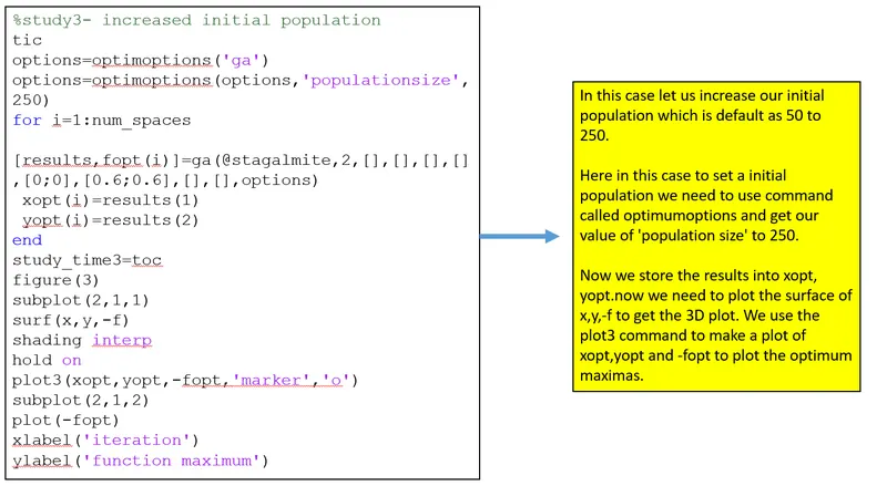
%study3- increased initial population
tic
options=optimoptions('ga')
options=optimoptions(options,'populationsize',250)
for i=1:num_spaces
 [results,fopt(i)]=ga(@stagalmite,2,[],[],[],[],[0;0],[0.6;0.6],[],[],options)
 xopt(i)=results(1)
 yopt(i)=results(2)
end
study_time3=toc
figure(3)
subplot(2,1,1)
surf(x,y,-f)
shading interp
hold on
plot3(xopt,yopt,-fopt,'marker','o')
subplot(2,1,2)
plot(-fopt)
xlabel('iteration')
ylabel('function maximum')
OUTPUT:
STUDY 1-UNBOUNDED
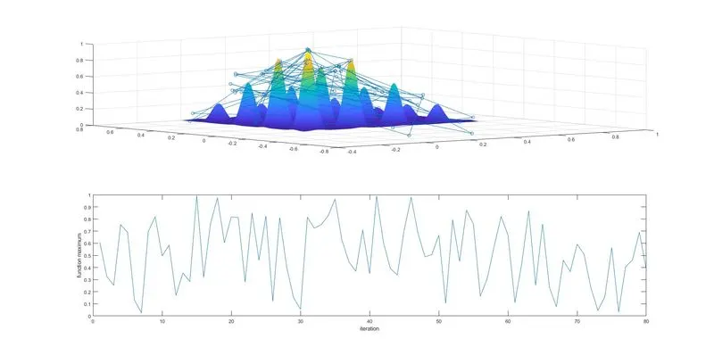
Here we can see the optimal values of x&y which is falling away the stagalmite surface.Here we failed to reach global maxima in this case.
and study time we get here is 2.9734s.
STUDY 2-BOUNDED
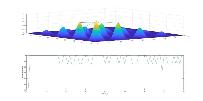
Here optimum values are within the limit but are not giving maximum values.
And study time we get here 4.0288s which is more than above study.
STUDY 2:iNCREASE IN POPULATION
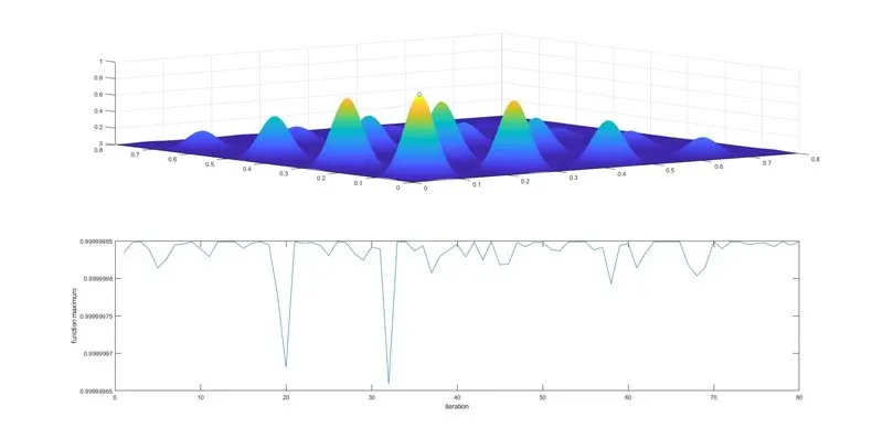
By increasing the size of population of ga so there is increase in accuracy of algorithm.
Here we observe study time more than above two studies is 13.0880.