Week 3 - Solving second order ODEs

Aim:to write a program for simulation of pendulum.

Theory:A pendulum is a body suspended from a fixed side which is swing back and forth under the influence og gravity.

for simulation of pendulum require second order eqn.

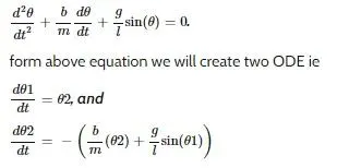
codes for calling a function

function[dtheta_dt]=ode_func(t,theta,b,g,l,m)
theta1=theta(1)
theta2=theta(2)
dtheta1_dt=theta2;
dtheta2_dt=-(b/m)*theta2-(g/l)*sin(theta1);
dtheta_dt=[dtheta1_dt;dtheta2_dt];
end

code for plotting a graph angular velocity vs angular displacement

clear all 
close all
clc

%inputs
b=0.05;
g=9.8;
l=1;
m=1;

%initial condition
theta_0=[0;5];
%time points
t_span=linspace(0,10,500);

%ode solve
[t,results]=ode45(@(t,theta)ode_func(t,theta,b,g,l,m),t_span,theta_0);
%plotting results
plot(t,results(:,1));
hold on
plot(t,results(:,2));
grid on
ylabel('angular velocity');
xlabel('angular displacement');

below is output

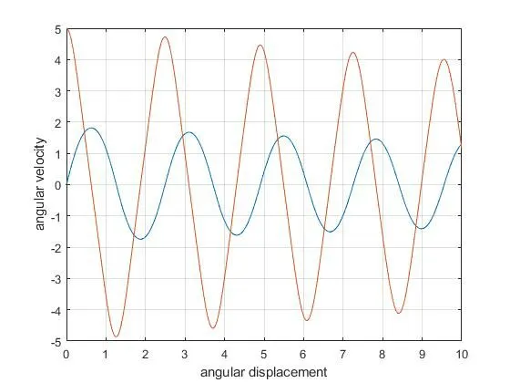
from the graph clearly shows that damping coefficient increases damping effect so there will be more to and fro.

creating a program for simulation of pendulum

clear all 
close all
clc

%inputs
b=0.05;
g=9.8;
l=1;
m=1;

%initial condition
theta_0=[0;5];
%time points
t_span=linspace(0,10,500);

%ode solve
[t,results]=ode45(@(t,theta)ode_func(t,theta,b,g,l,m),t_span,theta_0);
%plotting results
plot(t,results(:,1));
hold on
plot(t,results(:,2));
grid on
ylabel('angular velocity');
xlabel('angular displacement');

%simulation of pendulum

Ct=1;
for i=1:length(results(:,1))
    x0=0;
    y0=0;
    x1=l*sin(results(i,1));
    y1=-l*cos(results(i,1));
    plot([-0.5,0.5],[0,0],'linewidth',4,'color','g');
    line([x0 x1],[y0 y1],'linewidth',3,'color','r');
    hold on
    plot(x1,y1,'o','markers',20,'markerfacecolor','b');
    grid on
    axis([-3 3 -3 3]);
    pause(0.01);
    
    hold off;
    M(Ct)=getframe(gcf);
    Ct=Ct+1;
   
end
%creating  movie
movie(M)
videofile = VideoWriter('ode_2.avi');
open(videofile)
writeVideo(videofile,M)
close(videofile)

sir below is the google drive link for simulation of pendulum

https://drive.google.com/file/d/1YdQm66HdGEUMlFjU-RX2JA3yxE4hBInT/view?usp=sharing