Week 4.1 - Genetic Algorithm

giving values for x and y between 0 and 0.6

and number of itertions be 50

clear all
close all
clc         
%defining our search point
num_cases = 50;
x = linspace(0,0.6,150);
y = linspace(0,0.6,150);

now we make a 2d array of x and y using meshgrid command

%creating a 2Dimensional meshgrid
[xx yy] = meshgrid(x,y);

% evaluating the stalgamite function
for i = 1:length(xx)                
  for  j = 1:length(yy)
    input_vector(1)=xx(i,j);
    input_vector(2)=yy(i,j);
    f(i,j) = stalagmite(input_vector);
  end
end

now we create a function file for stalagmite function and gives the output as -f since the ga only gives the minimum value -f automatically becomes the maximum

function f = stalagmite(input_vector)

x = input_vector(1);
y = input_vector(2);

f1x = (sin(5.1*pi*x+0.5))^6;
f1y = (sin(5.1*pi*y+0.5))^6;
f2x = exp((-4*log(2)*(x-0.067)^2)/0.64);
f2y = exp((-4*log(2)*(y-0.067)^2)/0.64);

f =-(f1x*f1y*f2x*f2y);
end

now first study

%study 1 statistical behavior

tic
for k=  1:num_cases
[inputs,fopt(k)] = ga(@stalagmite,2);
xopt(k)=inputs(1);
yopt(k)=inputs(2);
end

study_time1 = toc

figure(1);  
surfc(xx,yy,-f)
shading interp
hold on
grid on
title('stalagmite plot')
xlabel('iterations');
ylabel('function_minimum');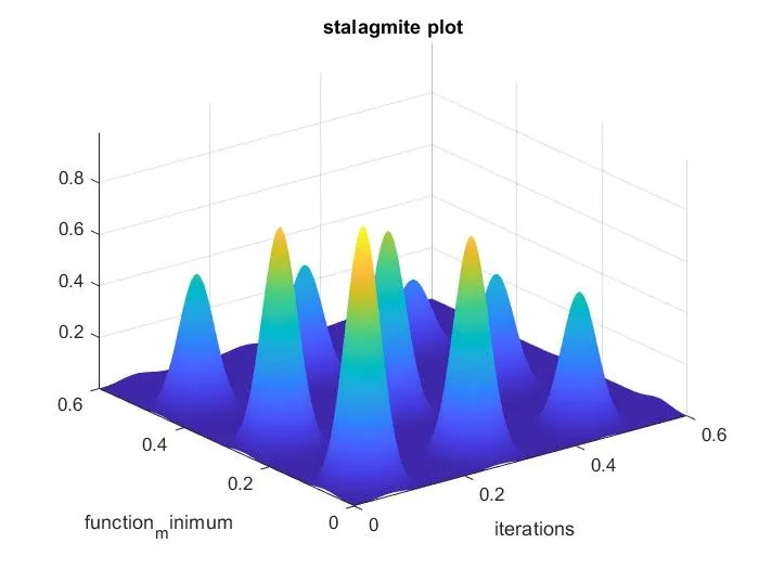   

figure(2)
subplot(2,1,1)
surfc(xx,yy,-f)
shading interp
hold on
plot3(xopt,yopt,-fopt,'marker','o','MarkerSize',4,'markerfacecolor','g');
subplot(2,1,2);
plot(-fopt)
title('iterations')
xlabel('iterations');
ylabel('function_minimum');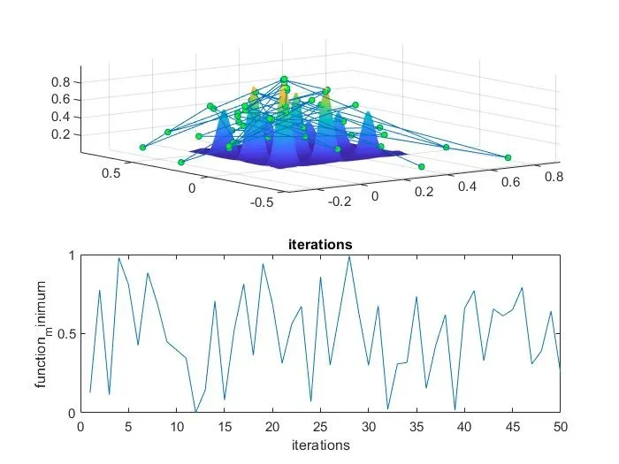   

here we can see that the optimal value went outside the value of x and y

so we couldnt find the global maxima

time taken for the study = 2.85s

2nd study

%2nd case study with upper and lower bounds
tic
for s = 1:num_cases
    [inputs,fopt(s)]= ga(@stalagmite,2,[],[],[],[],[0,0],[0.6,0.6]);
    xopt2(s)=inputs(1);
    yopt2(s)=inputs(2);
end
study_time2 = toc
figure(3);
subplot(2,1,1);
surfc(xx,yy,-f);
shading interp;
hold on
plot3(xopt2,yopt2,fopt,'marker','o','MarkerSize',4,'markerfacecolor','g');
title('bounded input width');
subplot(2,1,2);
plot(-fopt);
xlabel('iterations');  
ylabel('function_minimum');  

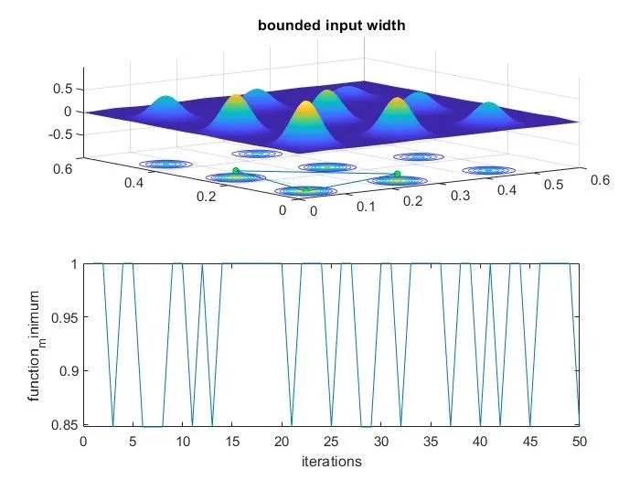
here the upper and lower bounds of x and y have been specified

here we couldnt get the exact maxima values

time taken = 3.06s

now study 3

here we increse the initial population size to 350

%study 3 increasing ga iterations
options=optimoptions('ga');
options=optimoptions(options,'PopulationSize',350);
for m = 1:num_cases
    [inputs,fopt(m)] = ga(@stalagmite,2,[],[],[],[],[0,0],[0.6,0.6],[],[],options);
xopt3(m)=inputs(1);
yopt3(m)=inputs(2);
end
study_time3 = toc
figure(4)
subplot(2,1,1);
surfc(xx,yy,-f);
shading interp;
hold on
plot3(xopt3,yopt3,-fopt,'marker','o','MarkerSize',4,'markerfacecolor','g');
title('unbounded inputs');
subplot(2,1,2); 
plot(-fopt);
xlabel('iterations');
ylabel('function_minimum');    

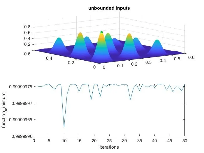
by incresing the initial population size of the ga, we can increase the accuracy of the ga

the global maxima has been found

time taken = 16.77s