Week 4.1 - Genetic Algorithm
Genetic Algorithms:
Inspired from the Darwin's theory of genetic, genetic algorithms reflect the process of natural selection where the process natural selection where the fittest individuals are individuals are selected for producing a strong off-spring for next generation.
The algorithm creates a ranom initial population. It continues to create generations of new population using the elements from the current generation.
To create a new generation, the algorithm:
i.)Evaluates the fitness score of each individual element of the population.
ii.) The members with the best fitness value are the elite an they naturally progress to the next generation.
iii.) Based on the limits and expectation values, select members are chosen as the parents for next generation
iv.)Then these parents produce children either through mutation, where random changes are made to the parent or cross-over , where the entries of both the parents are combined to form a ne child.
v.) This process continues until the end-criterion is reached, either through limiting the number of generations, time taken to calculate the optimum solution or a certain fitness limit is reached.
One of the most important aspects of genetic algorithms is the fitness function. It has to be optimized to avoid producing biased solutions which could lead to awkward unecessary solutions.
We can control the reproduction by choosing the fraction of children generated by cross-over in the pool other than individual elite children.
GA almost always provides a set of solutions without any derivative knowledge, which could be a good starting point. With end-criterion, we'll always get a solution irrespective of the fact whether the solution is optimal or not.
The larger the populations and the variables describing the problems, the better the performance of the Genetic algorithm.
With increase in population size, the computation time can drastically increased. The fitness value of an elite child is not carried onto the next generation and is calculated repeatedly making it a deterministic problem and also increasing the computation time by repeating redundant calculations.
It is dependent on efinition of problems and variables for optimal solution.
Syntax of GA:
[x,fval]=(fun,nvars,A,b,[],[],lb,ub,nonlcon,IntCon,options)
i.) x is the location of the minima point
ii.) fval is value of the optimal solution
iii.) fun is the function to be called to find out the optimal point for. Stalagmite function in this case.
iv.)nvars is number of variables used, we use 2 in this case.
v.)A,b and [],[] are inequalty conditions that are present in the function.
vi.)lb,ub is the upperbound and lowerbound of the function.
vii)nonclon is used for non linear constraints that represent inequalities and equalities.
viii.) Intcon is the condition to get an integral condition
ix.) Options are to execute en conditions, we limit the number of generations.
Code:
i.) We define the stalagmite function.
ii.) we define the each space x,y and create a mesh grid(array), an array of two variables.
iii.) We input the mesh grid values appropriately into the stalagmite function to get the appropriate curve.
iv.)Now that we have stalagmite curves, which have several peaks, we find the global maxima of the function using ga function and input the values appropriately as mentioned in the syntax.
v.) GA always finds the global minima, so we flip the sign of the function an find the minima. on flipping it again, the minima point(after flipping the first time) becomes the maximum point again. this is to simply find the minima of a flipped function, which would otherwise be the maxima.
vi.)we repeat this process for bounded inputs, unbouned inputs and for multiple generations case.
Code:
Unbounded case
clear all
close all
clc


%search space

x= linspace(0,0.6,150);
y= linspace(0,0.6,150);
[X,Y]=meshgrid(x,y);

count=50;%defining the number of iterations

%Stalagmite surface plot


for i=1:length(x)

    for j=1:length(y)

        input(1)=X(i,j);
        input(2)=Y(i,j);

        f(i,j)=stalagmite(input);
    end
end

F=-f;

surface(X,Y,F)
shading interp
hold on;


%studying statistical behavior for 50 iterations without any bounds

tic

for i=1:count

    [inputs,fopt(i)]=ga(@stalagmite,2);

    xopt(i)=inputs(1);
    yopt(i)=inputs(2);
end

Fopt=-fopt;
time_1=toc;

figure(1)

subplot(2,1,1)

surface(X,Y,F)
shading interp
hold on

plot3(xopt,yopt,Fopt,'marker','o','markersize',2,'markerfacecolor','r')

xlabel('X')
ylabel('Y')
title('stalagmite model and GA solutions')

subplot(2,1,2)

plot(Fopt)

xlabel('iterations')
ylabel('GA solutions')
Results:
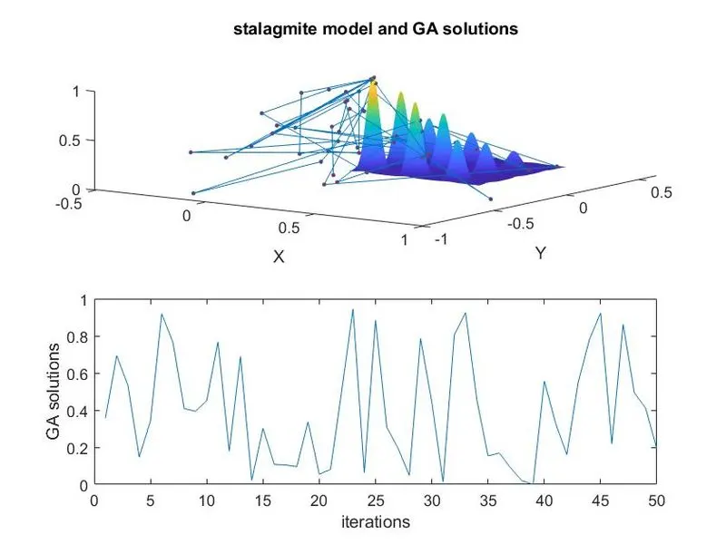
We can see that this is not optimal since the GA solutions are random and mapped outside the stalagmite function which is not ideal.
Bounded case:
%with boundation

clear all
close all
clc


%search space

x= linspace(0,0.6,150);
y= linspace(0,0.6,150);
[X,Y]=meshgrid(x,y);

count=50;%defining the number of iterations

%Stalagmite surface plot


for i=1:length(x)

    for j=1:length(y)

        input(1)=X(i,j);
        input(2)=Y(i,j);

        f(i,j)=stalagmite(input);
    end
end

F=-f;

surface(X,Y,F)
shading interp
hold on;


%studying statistical behavior for 50 iterations without any bounds

tic

%options = optimoptions('ga','MaxGenerations',300,'MaxStallGenerations',Inf,'PlotFcn',@gaplotbestf);

for i=1:count


    [inputs,fopt(i)]=ga(@stalagmite,2,[],[],[],[],[0;0],[0.6;0.6],[],[]);

    xopt(i)=inputs(1);
    yopt(i)=inputs(2);
end

Fopt=-fopt;
time_1=toc;

figure(1)

subplot(2,1,1)

surface(X,Y,F)
shading interp
hold on

plot3(xopt,yopt,Fopt,'marker','o','markersize',2,'markerfacecolor','r')

xlabel('X')
ylabel('Y')
title('stalagmite model and GA solutions')

subplot(2,1,2)

plot(Fopt)

xlabel('iterations')
ylabel('GA solutions')
Results:
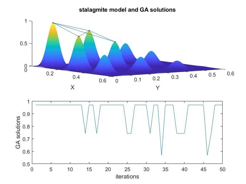
Well, this is better than the previous case, we could achieve the solutions within the stalagmite boundaries but this is still not ideal. It does not represent a single global maxima but rather four peaks
Final case with forcing the number of generations:
%with boundation

clear all
close all
clc


%search space

x= linspace(0,0.6,150);
y= linspace(0,0.6,150);
[X,Y]=meshgrid(x,y);

count=5;%defining the number of iterations

%Stalagmite surface plot


for i=1:length(x)

    for j=1:length(y)

        input(1)=X(i,j);
        input(2)=Y(i,j);

        f(i,j)=stalagmite(input);
    end
end

F=-f;

surface(X,Y,F)
shading interp
hold on;


%studying statistical behavior for 50 iterations without any bounds

tic

options = optimoptions('ga','MaxGenerations',700,'MaxStallGenerations',Inf,'PlotFcn',@gaplotbestf);

for i=1:count


    [inputs,fopt(i)]=ga(@stalagmite,2,[],[],[],[],[0;0],[0.6;0.6],[],[],options);

    xopt(i)=inputs(1);
    yopt(i)=inputs(2);
end

Fopt=-fopt;
time_1=toc;

figure(1)

subplot(2,1,1)

surface(X,Y,F)
shading interp
hold on

plot3(xopt,yopt,Fopt,'marker','o','markersize',2,'markerfacecolor','r')

xlabel('X')
ylabel('Y')
title('stalagmite model and GA solutions')

subplot(2,1,2)

plot(Fopt)

xlabel('iterations')
ylabel('GA solutions')
Results:
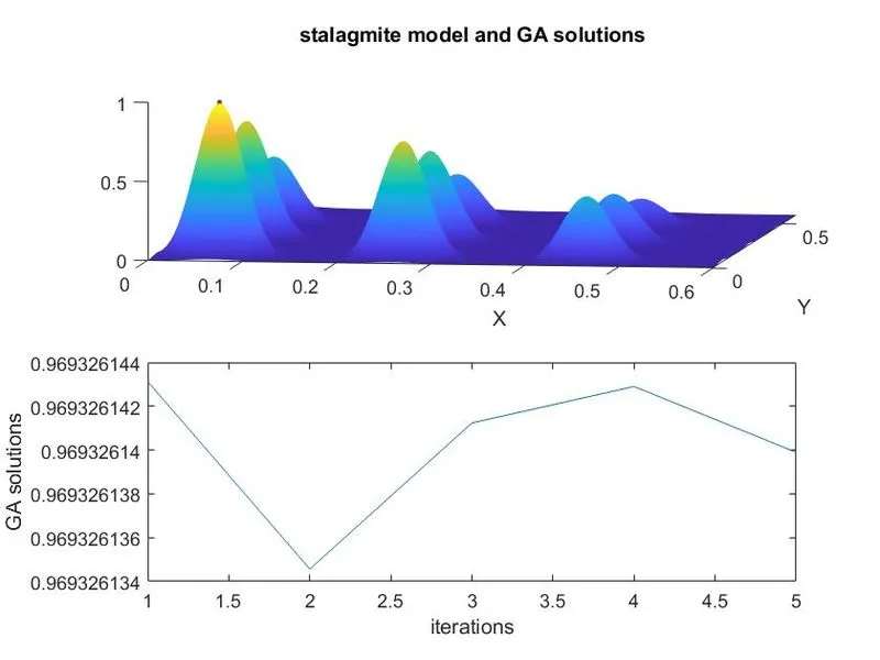
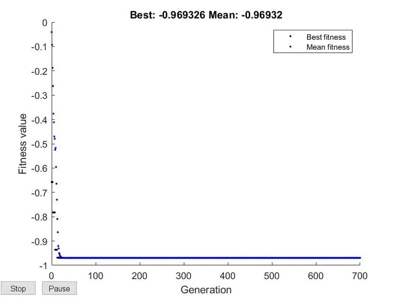
We see that by forcing to create more generations, we are getting solutions closer and closer to the global maxima.We finally attain the global value.