Project 2 - Rankine cycle Simulator
Objectives:
i.) Simulating Rankine cycle using MATLAB.
ii.) Extracting properties of water and steam from XSteam package.
iii.)Calculating and plotting all the states of the cycle.
Rankine cycle:
It is an idealized thermodynamic cycle which describes how heat engines like steam turbines extract mechanical work from fluid moving between heat source and heat sink while undergoing phase changes.
Power of Rankine cycle depends on temperature difference between the heat source and sink. Larger difference will result in higher extraction of mechanical power with higher efficiency. Unlike Carnot cycle, where the efficiency is only dependent on the temperature difference between the source and sink, Rankine cycles efficiency is depenent on the heat of vaporization of the liquid.
So, there is a need for supercritical fluids to be used and high performance materials in the turbine to withstand such temperatures and pressure ithout deteriorating.
Rankine Cycle has 4 steps:
i.) The working fluid is heated at the constant pressure where the liquid(water) converts into vapour.
ii.) Then it undergoes reversible adiabatic expansion, here it performs mechanical work by driving the turbine.
iii.) The fluid then cools at constant presure, where it converts to liquid.
iv.) It then undergoes aiabatic compresion and and is pumped back into the boiler.
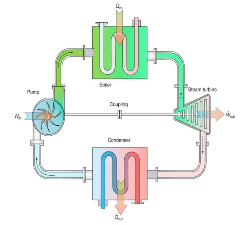
source:[1]
Code explanation:
i.) To escribe the rankine cycle, we need extract steam and water properties at different temperatures and pressure. we get this data using the XSteam package where we can get the entropy, enthalpy, temperature and volume data based on the states.
ii.) We enter the pressure and temperature at the inlet an pressure at the turbine outlet/condenser inlet.
iii.) Using the available input data, thermo dynamic relations and the XSteam library,we calculate all the state points of the rankine cycle.
iv.) Using the derived state points, we find out the work done by turbine, work done by the pump and the net work one by the cycle and efficiency. we also measure the specific steam consumption which is nothing but steam consumed per unit output of power.
v.) saturation liquid an gas data is extracted and plotted on the curve.
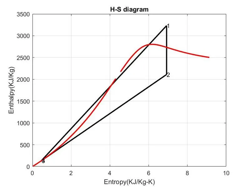
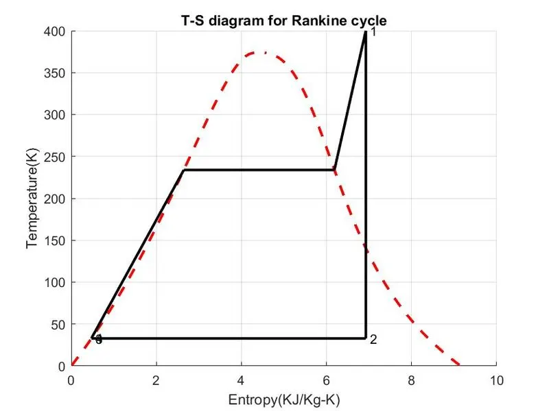
vi.) we then plot entropy vs temperature an enthalpy vs entropy plot.
Code:
clear all
close all
clc

%description

fprintf('Rankine Cycle Simulator');

fprintf('\n \n \n')

fprintf('1-2 ---> Isentropic expansion in the turbine \n');
fprintf('2-3 ---> Heat rejection by the turbine at constant pressure \n');
fprintf('3-4 ---> Isentropic compression in the pump \n');
fprintf('4-1 ---> Heat addition by the boiler at constant pressure \n \n \n');

%Input Pressure and Temperature

p1=input('Enter the pressure at the Turbine inlet: ');
T1=input('Enter the temperature at the Turbine inlet: ');
p2=input('Enter the pressure at the condenser/Turbine outlet: ');

%Calculating Enthalpy and specific entropy at each state

h1= XSteam('h_pT',p1,T1);%function of pressure and temperature
s1=XSteam('s_ph',p1,h1);%function of pressure and enthalpy

%print results at state 1

fprintf('results at state 1 \n \n')

fprintf('\n Pressure(p1) : %f bar',p1);
fprintf('\n Temperature(T1): %f Celsius',T1);
fprintf('\n Enthalpy : %f KJ/Kg',h1);
fprintf('\n Specific Entropy:%f KJ/kg-K \n \n',s1);


%state 2- Enthalpy, Temperaure, Specific Entropy

%it is at constant pressure,so we need to find temperature

s2=s1;%Isentropic step 1-2

T2=XSteam('T_ps',p2,s2);%T_ps is temperature as a function of pressure and entropy

s_liquid2=XSteam('sL_p',p2);%Saturated liquid entropy
s_vapour2=XSteam('sV_p',p2);%Saturated Vapour entropy

%enthalpies

h_vapour2=XSteam('hV_p',p2);%Saturated vapour enthalpy
h_liquid2=XSteam('hL_p',p2);%saturated liquid enthalpy


%Vapour fraction

X_2= ((s2 - s_liquid2)/(s_vapour2-s_liquid2));

h2= h_liquid2 + (X_2*(h_vapour2-h_liquid2));%Enthalpy at second state

V2= XSteam('v_ph',p2,h2);%Specific volume as a function of pressure and enthalpy

fprintf(' Results at state point 2 \n \n')
fprintf(' \n Pressure at state 2: %f',p2);
fprintf(' \n Temperature at state 2:%f Celsius',T2);
fprintf(' \n Specific volume at state 2: %f m^3/kg',V2);
fprintf(' \n Enthalpy at state 2: %f KJ/kg',h2);
fprintf(' \n Specific entropy at state 2: %f KJ/kg-K \n \n',s2);


%now at state 3, we reach state 3 by rejecting heat from state 2 at
%constant pressure.

T3= T2;
p3=p2;

s3= XSteam('sL_p',p3);%Entropy at state 3
h3= XSteam('hL_p',p3);%Enthalpy at state 3
V3= XSteam('vL_p',p3);%Specific volume at state 3
T2=T3;

fprintf(' Results at state point 3 \n \n')
fprintf(' \n Pressure at state 3: %f',p3);
fprintf(' \n Temperature at state 3:%f Celsius',T2);
fprintf(' \n Specific volume at state 3: %f m^3/kg',V3);
fprintf(' \n Enthalpy at state 3: %f KJ/kg',h3);
fprintf(' \n Specific entropy at state 3: %f KJ/kg-K \n \n',s3);


%Variables for stage 4

s4=s3;
V4=V3;
p4=p1;

h4=XSteam('h_ps',p4,s4);
T4=XSteam('T_ps',h4,s4);


fprintf(' Results at state point 4 \n \n')
fprintf(' \n Pressure at state 4: %f',p4 );
fprintf(' \n Temperature at state 4:%f Celsius',T4);
fprintf(' \n Specific volume at state 4: %f m^3/kg',V4);
fprintf(' \n Enthalpy at state 4: %f KJ/kg',h4);
fprintf(' \n Specific entropy at state 4: %f KJ/kg-K',s4);


%Turbine does some work, it is the difference in enthalpies
Wt=h1-h2;

%work done by the pump

Wp= h4-h3;

%net work done, is (h1+h3)-(h2+h4) which is wt-wp

W_net= Wt-Wp;


%heat added in the boiler
q_in= h1 - h4;

%heat rejected in the condenser

q_out= h2-h3;

%Thermal efficiency

n=(W_net/q_in)*100;

SSC= 3600/Wt;%specific steam consumption

fprintf('  Final output \n \n')
fprintf(' \n Work output by Turbine: %f KJ/kg',Wt );
fprintf(' \n Work input by the pump:%f  KJ/kg',Wp);
fprintf(' \n Net work done: %f  KJ/kg',W_net);
fprintf(' \n Heat added in the boiler: %f KJ/kg',q_in);
fprintf(' \n Heat rejected in the condenser: %f KJ/kg',q_out);
fprintf(' \n Thermal efficiency: %f percent',n);
fprintf(' \n Specific steam consumption: %f Kg/kWh',SSC);


%plotting

temp= linspace(1,T1,1000);

for i=1:length(temp)

    h_liquid(i)= XSteam('hL_T',temp(i));
    h_vapour(i)= XSteam('hV_T',temp(i));
    s_Liquid(i)= XSteam('sL_T',temp(i));
    s_vapour(i)= XSteam('sV_T',temp(i));
end

figure(1)

hold on
plot(s_Liquid, temp,'linewidth',2,'linestyle','- -','color','r');
plot(s_vapour, temp,'linewidth',2,'linestyle','- -','color','r');

grid on


%process 1-2
plot([s1 s2], [T1 T2], 'k', 'linewidth',2)
hold on

title('T-S diagram for Rankine cycle')
xlabel('Entropy(KJ/Kg-K)')
ylabel('Temperature(K)')

%process 2-3

plot([s2 s3],[T2 T3],'linewidth',2,'color','k')

hold on

%process 3-4

plot([s3,s4],[T3,T4],'linewidth',2,'color','k')

%heat added by the boiler

tp=XSteam('TSat_p',p4);
sp=XSteam('sL_T',tp);

plot([s4,sp],[T4,tp],'linewidth',2,'color','k')

hold on

tq=tp;

sq=XSteam('sV_T',tp);

plot([sp,sq],[tp,tq],'linewidth',2,'color','k')
hold on

plot([sq,s1],[tq,T1],'linewidth',2,'color','k')

%Indicate state with numbers
text(s1,T1,' 1');
text(s2,T2,' 2');
text(s3,T3,' 3');
text(s4,T4,' 4');

%plot for the enthalpy vs entropy

figure(2)

plot([s1,s2],[h1,h2],'linewidth',2,'color','k')

grid on
title('H-S diagram')
xlabel('Entropy(KJ/Kg-K)')
ylabel('Enthalpy(KJ/Kg)')

hold on

plot([s2,s3],[h2,h3],'linewidth',2,'color','k')
hold on
plot([s3,s4],[h3,h4],'linewidth',2,'color','k')
hold on
plot([s4,s1],[h4,h1],'linewidth',2,'color','k')


%plot for liquid and vapour saturation curve

temperature=linspace(1,T1,1000);

for j=1:length(temperature)
    h_l(j)= XSteam('hL_T',temperature(j));
end

for j=1:length(temperature)

    h_v(j)=XSteam('hV_T',temperature(j));
end

plot(s_Liquid,h_l,'linewidth',2,'color','r')
hold on
plot(s_vapour,h_v,'linewidth',2,'color','r')

%Indicate state with numbers

text(s1,h1,'1');
text(s2,h2,'2');
text(s3,h3,'3');
text(s4,h4,'4');


%
Sources:
[1]: Ibrahim Dincer,
1.6 Exergy,
Editor(s): Ibrahim Dincer,
Comprehensive Energy Systems,
Elsevier,
2018,
Pages 212-264,
ISBN 9780128149256,
https://doi.org/10.1016/B978-0-12-809597-3.00106-1.
(https://www.sciencedirect.com/science/article/pii/B9780128095973001061)
Abstract: This contribution focuses on exergy as a potential field of thermodynamics, which aims to design, analyze, assess, evaluate, and improve thermodynamic systems. These thermodynamic systems are classified into categories here as closed and open systems for exergy analysis. Numerous example problems, and case studies are presented to highlight the importance of exergy and its use for closed and open systems. Furthermore, several key aspects and concepts of exergy and exergy-related parameters are introduced and discussed in comparison with the corresponding energy and energy-related parameters.
Keywords: Analysis; Design; Efficiency; Energy; Energy systems; Environment; Exergy destruction; Exergy; Thermodynamics