Week 4.1 - Genetic Algorithm

Aim- To write a matlab program to calucate the gobal maxima of the stalagmite function and explain the syntex genitic algorithm (ga).

objectives-

* To write a code of matlab to optimize the stalagmite function and explain the gobal maxima of the function.

* To explain the expain the genitic algorithm and the syntax of the ga in matlab .

* Tob plot the graphs of all three studies of the global maxima.

Theory-

optimization-

optimization is an area of study which is used to maximum or minimum the particular function,which depends upon mulitiple parameters to get the desired output

stalagmite-

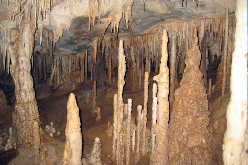
stalagmite mathematical model used to develop the local maximum or minimum hear to determine the optimiza solution of the function we are using the genetic algorithm techinque

genitic algorithm-

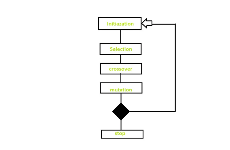
gentic algorithm is an optimization techique to slove non linear &non-differential optimization problem the name come from using evolution biology technique (darwin's theroy of evolution)

it is starts with an initial generation of candidate solution that is tested against the objective function.subsequent generation evolves from the frist throught selection,crossover,mutation.which continous until the cycle stop with the true value

selection-

In this we are selecting the best performing bit strings from one generation to the next generation i.e based on the fitness

crossover-

Due to they perfromed well therfore taking comman between them to create a child.

mutation-

Taking parent and mutate certain variable and create a child based on mutation.

Equation used-

`f(x,y)=f1x,f2x,f1y,f2y`

`f1.x=[sin(5.1pix+0.5)]^6`

`f1.y=[sin(5.1piy+0.5)]^6`

`f2.x=[-4log(2)frac{(x-0.0667)^2}{0.64}]`

`f2.y=[-4log(2)frac{(y-0.0667)^2}{0.64}]`

Here x and y are variables

syntax referred for gentic algorithm-

in a main program we have to use the one dimensional array x and y with linspace command and as we know the x and y are the input arrayit does not defined the workspace of the gentic algoirithm

syntax Referred:

x= ga(fun,nvars)

x= ga(fun,nvars,A,b)

x= ga(fun,nvars,A,b,Aeq,beq)

x= ga(fun,nvars,A,b,Aeq,beq,lb,ub)

x= ga(fun,nvars,A,b,Aeq,beq,lb,ub,nonlcon)

x= ga(fun,nvars,A,b,Aeq,beq,lb,ub,nonlcon,options)

x= ga(fun,nvars,A,b,[],[],lb,ub,nonlcon,Intcon)

x= ga(fun,nvars,A,b,[],[],lb,ub,nonlcon,Intcon,options)

x= ga(problem)

[x,fval]= ga(_)

[x,fval,exitflag,output]= ga(_)

[x,fval,exitflag,output,population,scores]= ga(_)

procedure-

program:

plotting the gobal maxima

clear all
close all
clc
%definding our search space
x=linspace(0,0.6,150);
y=linspace(0,0.6,150);

%creating a 2D dimensional mesh
[xx yy]=meshgrid(x,y);

for i =1:length(xx)
    for j = 1:length(yy)
        input_vector(1)=xx(i,j);
        input_vector(2)=yy(i,j);
        f(i,j)= stalagmite(input_vector);
    end
end
%plotting
surf(xx,yy,f)
shading interp

[inputs,fval]=ga(@stalagmite,2);
xlabel('x value')
ylabel('y value')

Function

function [fx_y]=stalagmite(input_vector);
x=input_vector(1);
y=input_vector(2);

f1_x=[sin(5.1*pi.*x+0.5)].^6;
f1_y=[sin(5.1*pi.*y+0.54)].^6;
f2_x=exp(-4*log(2).*(((x-0.0667).^2)/0.64));
f2_y=exp(-4*log(2).*(((y-0.0667).^2)/0.64));
[fx_y]=(f1_x.*f1_y.*f2_x.*f2_y);
end

Here plotting the gobal maxima and finding the minimum of the ga

clear all
close all
clc
%defining the array
x=linspace(0,0.6,150);
y=linspace(0,0.6,150);
%creating a 2D dimensional mesh
[xx yy]=meshgrid(x,y);

for i =1:length(xx)
    for j = 1:length(yy)
        input_vector(1)=xx(i,j);
        input_vector(2)=yy(i,j);
        f(i,j)= stalagmite(input_vector);
    end
end


num_cases=50



%study_statistical behaviour
tic

for i=1:num_cases;
    [inputs,fopt(i)]=ga(@stalagmite,2);
    xopt(i)=inputs(1);
    yopt(i)=inputs(2);
end
study1_time=toc;

figure(1)

subplot(2,1,1);
hold on
surfc(x,y,f);
shading interp
plot3(xopt,yopt,fopt,'marker','o','markersize',6,'markerfacecolor','r');
title('unbounded inputs')
subplot(2,1,2);
plot(fopt);
xlabel('iteration')
ylabel('function maximum')

tic
%study statistical
for i=1:num_cases;
    [inputs,fopt(i)]=ga(@stalagmite,2,[],[],[],[],[0;0],[0.6;0.6])
    xopt(i)=inputs(1);
    yopt(i)=inputs(2);
end
study2_time=toc;

figure(2)
subplot(2,1,1);
hold on
surfc(x,y,f)
shading interp
plot3(xopt,yopt,fopt,'marker','o','markersize',6,'markerfacecolor','r');
title('bounded inputs')
subplot(2,1,2);
plot(fopt);
xlabel('iteration')
ylabel('function maximum')

% increasing ga iteration
options=optimoptions('ga')
options=optimoptions(options,'populationsize',300)

tic
%study statistical behaviour
for i =1:num_cases
    [inputs,fopt(i)]=ga(@stalagmite,2,[],[],[],[],[0;0],[0.6;0.6],[],[],options);
    xopt(i)=inputs(1);
    yopt(i)=inputs(2);
end
study3_time=toc
figure(3)
subplot(2,1,1)
hold on
surfc(x,y,f)
shading interp
plot3(xopt,yopt,fopt,'marker','o','markersize',5,'markerfacecolor','b')
subplot(2,1,2)
title('bounded inputs')
plot(fopt)
xlabel('iteration')
ylabel('function minumum')

results-

gobal maxima-

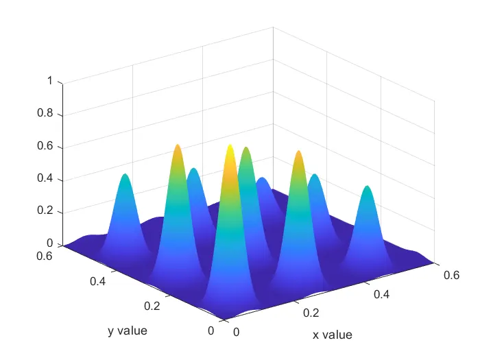
study1-

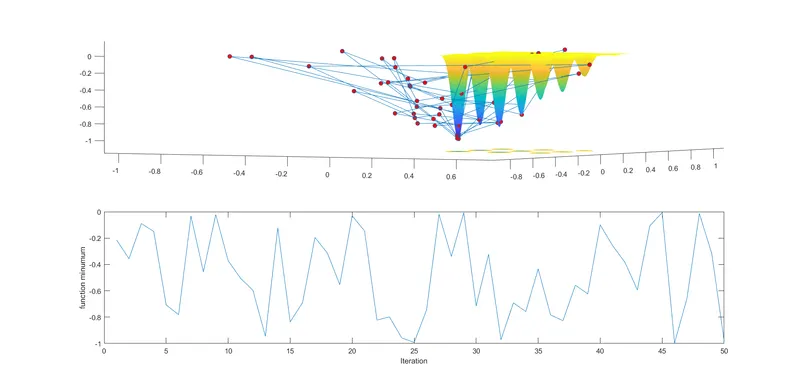
now we gwt the frist study we get mulitiple results,due to random sampling and maximum value changes from between 0.2 to 0.8,also time is taken to the frist study is 2.0536 seconds

study2-

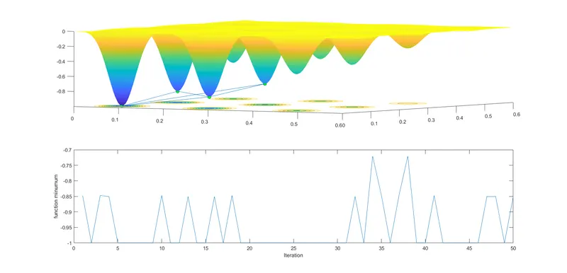
Here,maximum value is between 0.7 to 0.85 which is much less range.also time taken to the second study is 3.1061 seconds

study3-

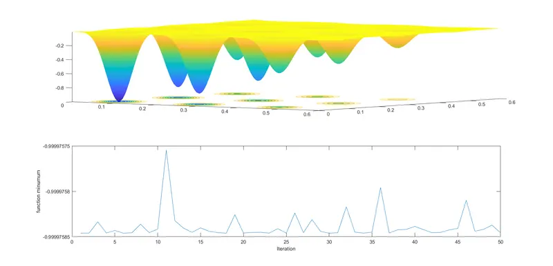
now,we get the most accurate result which is between 0.99997575 to 0.99997585.time is taken to the third study is 9.3573

error and correction-

The error happend due to the mistakes of the executing the program

after given the apropriate function the error was removed

conclusion-

Hence we able to opitimise the stalagmite funtion and find the gobal maxima of the function.

The ga is only used for the minimum function to the maximum function we inversed the maximum funtion