Week 3 - Solving second order ODEs

Aim-To solve the second order by using matlab that will simulate the pendulum motion and to create animation the motion of the pendulum

govering equation-

`frac {d^2theta} {dt^2} +frac {b}{m}frac{d theta}dt+frac{g}{l}sin theta=0`

the above equation-

b= damping coefficent

g=accelaration due to gravity(m/s2)

m=mass of the ball(kg)

l=length of the pendulum in m

`theta=theta1`

`frac{d theta}{dt}=frac{d theta1}{dt}=theta2`............(1)

`frac{d^2 theta}{dt^2}=frac{d}{dt}[frac{d theta1}{dt}]=frac{d}{dt} (theta2)`..............(2)

`frac{d^2theta}{dt^2}+frac{b}{m}frac{d theta}{dt}+frac{g}{l}sintheta=0`

`frac{d^2theta1}{dt^2}+frac{b}{m}frac{d theta1}{dt}+frac{g}{l}sintheta1=0`

from eq (1)&(2)

`frac{d theta2}{dt}+frac{b}{m}theta2+frac{g}{l}sintheta1=0`

`frac{d theta2}{dt}=-frac{b]{m} theta2-frac{g}{m}sintheta1`

`frac{d}{dt}[[theta1],[theta2]]=[[theta2],[-frac{b}{m}theta2-frac{g}{l}sintheta1]]`

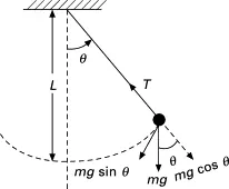
objectives-

* To slove the second order ODE with graph of velocity v/s displacement.

* To create the animation of the simple pendulum.

Theory-

fixed parameters-

b=0.05

m=1kg

g=9.81(m/s2)

l=1m

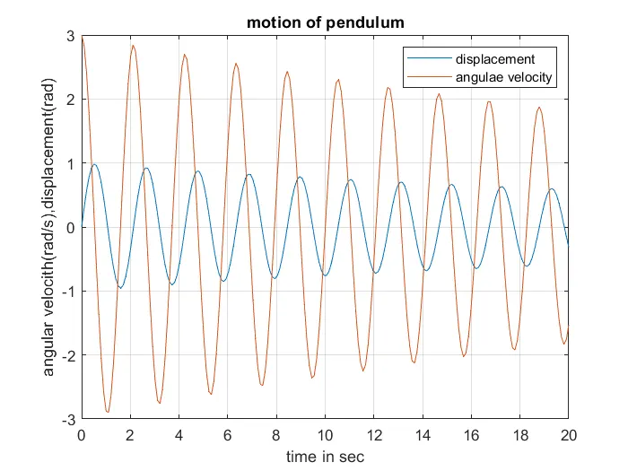
simulate the motion between 0-20sec,for angular displacement=0,angular velocity=3 rad/sec at time t=0and to and fro motion of the pendulum as a function time,to create a animation of the pendulum.

simple pendulum-

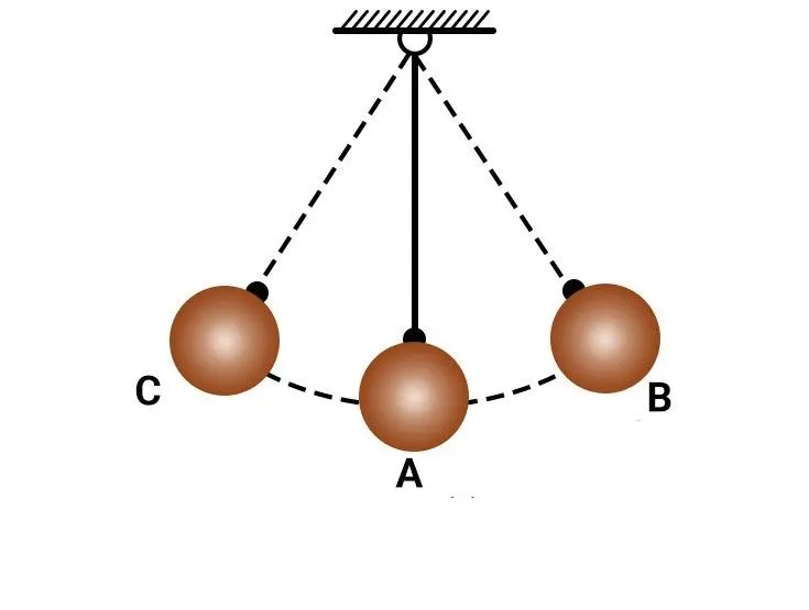
The simple pendulum is a idealized mathematical model of a pendulum.This ia a weigth on the end of amassless cord suspended from a pivot,without friction.when given an initial push,it will swing back and forth at a constant amplitude.Real pendulum are subject to friction and air drag,so amplitude of their swings declines.

procedure-

Matlab file-

1)code function of the ode45 main program

function [dtheta_dt]=ode_45(t,theta,b,g,m,l)

theta1=theta(1);
theta2=theta(2);

[dtheta1_dt]=theta2;
[dtheta2_dt]=-(b/m)*theta2-(g/l)*sin(theta1);

[dtheta_dt]=[dtheta1_dt;dtheta2_dt];
end

explanation-

1)The function name of the t,theta,b,g,m,l of the dtheta_dt

2)dtheta_dt is the by using the colume matrix [dtheta1_dt;dtheta2_dt]

2)main program-

clear all
close all
clc

% fixed parameters
%damping coefficent
b = 0.05;
%accelaration due to gravity(m/s^2)
g = 9.81;
%mass of the ball(kg)
m = 1;
%length of the pendulum(m)
l = 1;

%initial condition
theta_0 = [0;3];

%time point
t_span = linspace(0,20,200);

%solve ODE
[t,results]=ode45(@(t,theta) ode_fun(t,theta,b,g,m,l),t_span,theta_0);

%plotting angular velocity and displacement
figure(1)
plot(t,results (:,1));
hold on
plot(t,results (:,2));

xlabel('time in sec')
ylabel('angular velocith(rad/s),displacement(rad)')
legend('displacement','angulae velocity')
title('motion of pendulum')
grid on

%animation

ct=1;
for i =1:length(results(:,1))

    x0=0;
    y0=0

    x1=l*sin(results(i,l)+pi)
    y1=l*cos(results(i,l)+pi)
    figure(2)
    plot([x0 x1],[y0 y1],'-o','markersize',10,'markerfacecolor','r','markeredgecolor','r','linewidth',5);
    axis([-2 2 -2 2]);
    hold on
    plot([-1,1],[0,0],'linewidth',5,'color','[0 0.3 0]');
    M(ct)=getframe(gcf)
    hold off
    ct=ct+1;
end

%movie &videofile
movie(M)
videofile=VideoWriter('simple_pendulum.avi','uncompressed AVI')
open(videofile)
writeVideo(videofile,M)
close(videofile)

code explanation-

1)the given fixed parameters of the damping,gravity,mass,length of the pendulum

2) And initial condition of the angle and time is the theta_0,t_span.

3)slove the second order ODE of the by using of the ode45.

4)plotting the angular velocity and angular displacement.

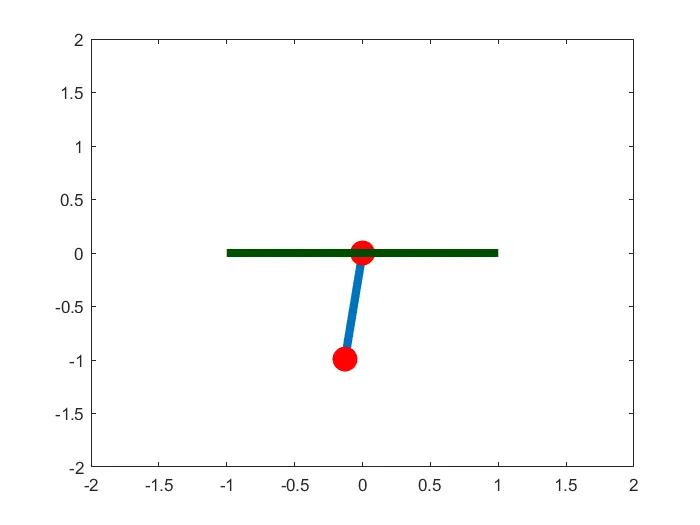
5)using the for loop to create a motion of the simple pendulum.

6)The pendulum as fixed coordinate x0,y0 and x1,x2

6)finally we can save a movie videofile in the .avi file .

figure(1)

figure(2)

Animation-

https://youtu.be/pfpx5-OdPZs

conclusion-

1)The graph of displacement and angular velocity is plotting in velocity v/s time diagram.

2)Animation of simple pendulum is created