Week 4.1 - Genetic Algorithm

AIM: To write a code in MATLAB to optimise the stalagmite function and find the global maxima of the function.

OBJECTIVE: The objective of this report is to optimise the stalagmite function by coding the program with help of genetic algorithm in MATLAB and explain the concept of genetic algorithm and also explain the syntax for 'ga' in MATLAB.

STALAGMITE FUNCTION:

• Stalagmite function is a mathematical model that helps to generate maximas and minimas.
• Global maxima is a maximum peak value in entire function and global minima is a minimum peak value in entire function. But local maxima and local minima are multiple number of values. Optimisation is finding of maxima and minima in particular function but in genetic algorithm, its only to find minima.

GENETIC ALGORITHM:

• A genetic algorithm is inspired by Charles Darwin’s theory of natural evolution. This algorithm reflects the process of natural selection where the fittest individuals are selected for reproduction in order to produce offspring of the next generation.
• A genetic algorithm (GA) is a method for solving both constrained and unconstrained optimization problems based on a natural selection process that mimics biological evolution. The algorithm repeatedly modifies a population of individual solutions. At each step, the genetic algorithm randomly selects individuals from the current population and uses them as parents to produce the children for the next generation. Over successive generations, the population "evolves" toward an optimal solution.

SYNTAX FOR GA IN MATLAB:

SYNTAX	EXPLAINATION
x = ga(fun, nvars)	Finds a local unconstrained minimum, x, to the objective function, fun. nvars is the dimension
x = ga(fun,nvars,A,b)	Finds a local minimum x to fun, subject to the linear inequalities A*x ≤ b. ga evaluates the matrix product A*x as if x is transposed (A*x').
x = ga(fun,nvars,A,b,Aeq,beq)	Finds a local minimum x to fun, subject to the linear equalities Aeq*x = beq and A*x ≤ b. (Set A=[] and b=[] if no linear inequalities exist.) ga evaluates the matrix product Aeq*x as if x is transposed (Aeq*x').
x = ga(fun,nvars,A,b,Aeq,beq,lb,ub)	Defines a set of lower and upper bounds on the design variables, x, so that a solution is found in the range lb ≤ x ≤ ub.
x = ga(fun,nvars,A,b,Aeq,beq,lb,ub,nonlcon)	Subjects the minimization to the constraints defined in nonlcon. The function nonlcon accepts x and returns vectors C and Ceq, representing the nonlinear inequalities and equalities respectively. ga minimizes the fun such that C(x) ≤ 0 and Ceq(x) = 0.
x = ga(fun,nvars,A,b,Aeq,beq,lb,ub,nonlcon,options)	It minimizes with the default optimization parameters replaced by values in options.

CODE:

close all

clear all

clc

 

%To Define the array x and y using linspace command

x=linspace(0,0.6,150);

y=linspace(0,0.6,150);

 

%To Define the 2d Array of x & y using meshgrid command

[xx,yy]=meshgrid(x,y);

 

tic

%solving the stalagmite function

for i=1:length(xx)

    for j=1:length(yy)

        input_vector(1)=xx(i,j);

        input_vector(2)=yy(i,j);

        f(i,j)=stalagmite_fun(input_vector);

    end

end

num_case=100;

 

%%CASE STUDY 1%%

for i=1:num_case

    [inputs,fopt(i)]=ga(@stalagmite_fun,2);

    xopt(i)=inputs(1);

    yopt(i)=inputs(2);

end

figure(1)

subplot(2,1,1)

surfc(xx,yy,f)

shading interp

hold on

plot3(xopt,yopt,fopt,'marker','o','markersize',5,'markerfacecolor','b')

subplot(2,1,2)

plot(fopt)

xlabel('Iterations')

ylabel('Function Maximum')

study1_time=toc

 

%%CASE STUDY 2%%

 tic

for i=1:num_case

    [inputs,fopt(i)]=ga(@stalagmite_fun,2,[],[],[],[],[0;0],[0.6;0.6]);

    xopt(i)=inputs(1);

    yopt(i)=inputs(2);

end

figure(2)

subplot(2,1,1)

surfc(xx,yy,f)

shading interp

hold on

plot3(xopt,yopt,fopt,'marker','o','markersize',5,'markerfacecolor','b')

subplot(2,1,2)

plot(fopt)

xlabel('Iterations')

ylabel('Function Maximum')

study2_time=toc

 

%%CASE STUDY 3%%

options = optimoptions('ga')

options = optimoptions(options,'populationSize',200)

 tic

for i=1:num_case

    [inputs,fopt(i)]=ga(@stalagmite_fun,2,[],[],[],[],[0;0],[0.6;0.6],[],[],options);

    xopt(i)=inputs(1);

    yopt(i)=inputs(2);

end

figure(3)

subplot(2,1,1)

surfc(xx,yy,f)

shading interp

hold on

plot3(xopt,yopt,fopt,'marker','o','markersize',5,'markerfacecolor','b')

subplot(2,1,2)

plot(fopt)

xlabel('Iterations')

ylabel('Function Maximum')

study3_time=toc

CODE EXPLANATION:

• The program is written to optimise the stalagmite function and finding of the global maxima of a function.
• First to define the array x and y using linspace command with 150 values between 0 to 0.6
• Later we considered the num cases as 100, for running GA 100 times and then code will calculate the study time for 100 iterations.
• Before starting the program we created function named. Stalagmite_fun as follows,

function [F]= stalagmite_fun(input_vector)

x=input_vector(1);

y=input_vector(2);

f1=(sin(5.1*pi.*x+0.5)).^6;

f2=(sin(5.1*pi.*y+0.5)).^6;

f3=exp(-4*log(2).*((x-0.0667)^2/0.64));

f4=exp(-4*log(2).*((y-0.0667)^2/0.64));

F=(f1.*f2.*f3.*f4);

end

• The following are the equations used as stalagmite function,

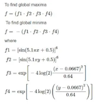
• To program the GA with Stalgmite function, three case studies are carried out.

CASE STUDY 1:

• In this case, we used the for loop as ga(@stalagmite) to find the statistical behaviour of function and also by using the tic and toc command we measured the time required for code to run. Then sub-plotted the figure along with the surface command to create 3D plot and shading with shading interp command.
• Secondly we used the plot3 command with (x,y,f) for multiple coordinates and titled the unbounded input commands and to further label the plot we use X label as Iterations and Y label as Function Maximum and then study1_time has been calculated.

CASE STUDY 2:

• In this case study, we have calculate the statistical behaviour of stalagmite function by setting up lower and upper bounds, with lb (x1,y1) is (0,0) and ub(x2,y2) is (0.6,0.6).
• With this change we found that there is increase in study time for optimization.
• Rest other steps are similar with CASE STUDY 1

CASE STUDY 3:

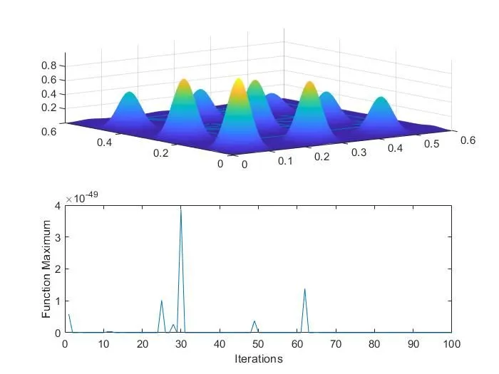
• In third case population size has been considered as 200; GA starts with random variable as there as 2 variables, we will be having 100 sets of 2 random variables.
• As we increase the population, we get global maxima.
• Rest other steps are similar with CASE STUDY 1 & 2.

CONCLUSION:

1. After significant iterations with num cases ga undergoes optimum value. i.e. global maxima can be found.
2. If we provide less iterations and run the program, ga may or may not able to find global maxima. But if number of iterations increases possibility of finding global maxima can also increases.
3. When population size increases with iteration, probability of global maxima can be optimise.
4. The plots are attached for reference.

Figure 1:

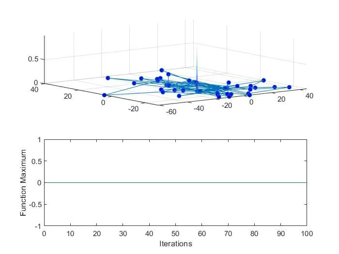
Figure 2:

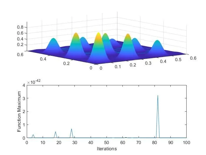
Figure 3:

RESULT:

Thus the global maxima of the stalagmite function is optimised using genetic algorithm in MATLAB

REFERENCES:

1. Genetic Algorithm - MATLAB & Simulink (mathworks.com)
2. Mathwork help