Project 2 - Rankine cycle Simulator

The Rankine Cycle Simulator

AIM: To create a Rankine Cycle Simulator using MATLAB.

OBJECTIVE:

1. To calculate each state points of the Rankine Cycle (any type of your choice) based on user inputs.
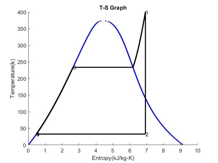
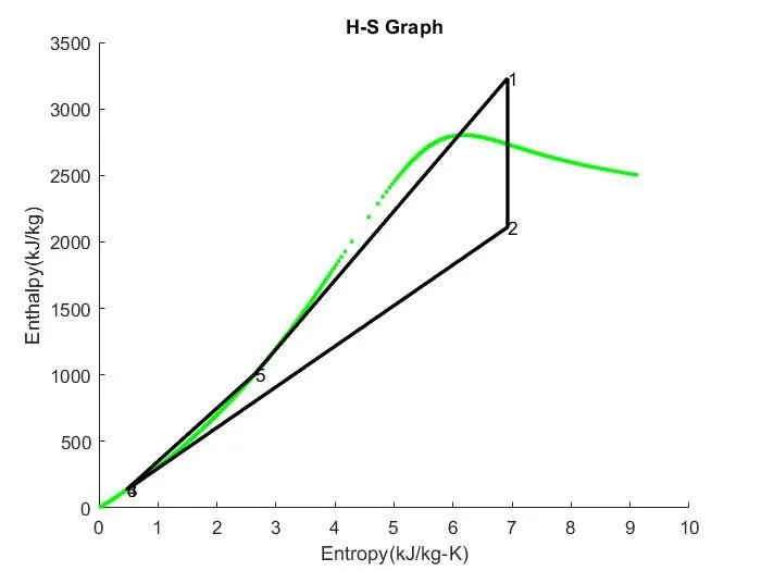
2. To plot the corresponding T-s and h-s plots for the given set of inputs.
3. To calculate Cycle Efficiency, Net Work & Back Work Ratio

THEORY:

1. The Rankine cycle describes the performance of steam turbine systems.
2. In general, the Rankine Cycleis an idealized thermodynamic cycle of a constant pressure heat engine that converts part of heat into mechanical work.
3. In this cycle the heat is supplied externally to a closed loop, which usually uses water (in a liquid and vapor phase) as the working fluid.
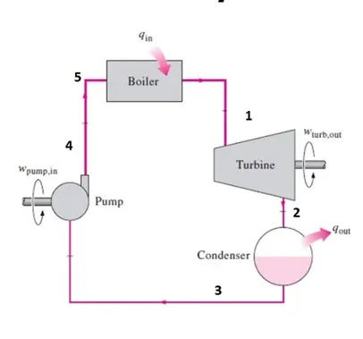
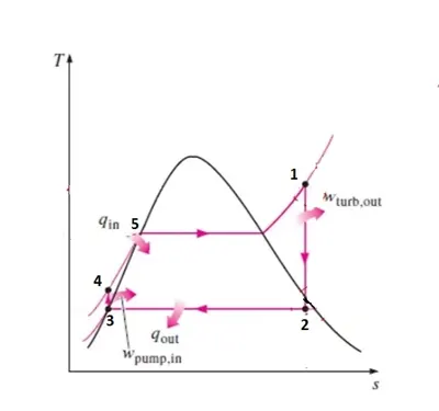
4. Following figure shows the arrangement of equipment in steam power plant based on Rankine Cycle; with Temperature - Entropy graph for the same.

Fig. 1. Schematic for Steam Power Plant	Fig. 2. Ideal Rankine Cycle (T-S Diagram)

5. Four processes of the Rankine cycle: (Let mass flow rate, m=1 kg/s)

• Isentropic Expansion Turbine (1-2): Superheated steam enters into the Turbine and expands isentropically resulting in the production of work. The shaft of the turbine is connected to the generator. This results in the production of electricity i.e Mechanical energy gets converted into electric energy.

Work produced by the turbine, W_T = (H1 − H2) kJ/kg

• Isobaric Heat Rejection in Condenser (2-3): The expanded vapour is then passed through a condenser, where it gets condensed and converts into liquid again. This liquid is again pumped to the boiler.

Heat Rejected by the Condenser, Qr = (H2 − H3) kJ/kg

• Isentropic Compression by the Pump (3-4): The water enters into the pump in a saturated state. Then the liquid is compressed isentropically until it meets the boiler pressure.

Work required by the pump is, Wp = (H4 – H3) kJ/kg

• Isobaric Heat Addition in the Boiler (4-5-1): The water enters into the boiler as compressed and leaves as superheated from the boiler. Thus the phase changes from liquid to vapour.

The heat supplied by the boiler is, Qs = (H1 – H4) kJ/kg

(Where, H=Enthalpy, T=Temperature, W=Work, Q=Heat)

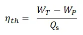
6. The Thermal efficiency of the Steam Cycle is given by,

6. Applying the Steady Flow Energy Equation (SFEE) to all the process, (neglecting the Friction losses and changs in Kinetic & Potential Energy),

• Wt=h1-h2 at Turbine
• Qr=h2-h3 at Condenser
• Wp=h4-h3 at Pump
• Qs=h1-h4 at Boiler

8. The Capacity of the Steam Plant is often expressed in terms of Steam Rate (SR) or Specific Steam Consumption (SSC), S. S. C. = 3600/(WT-Wp) kg/kWhr
9. Back Work Ratio shall be calculated as, B. W. R. = Wp/WT

CODE:

clear all
close all
clc
disp(' RANKINE CYCLE SIMULATOR ');
disp('1-2 is Isentropic Expansion in the Turbine');
disp('2-3 is Isobaric Heat Rejection by the Condenser');
disp('3-4 is Isentropic Compression in the Pump');
disp('4-5-1 is Isobaric Heat Addition by the Boiler');
fprintf('\n');
%Taking inputs from user
P1 = input('Enter the Pressure at the Turbine Inlet(in bar): ');
T1 = input('Enter the Temperature at the Turbine Inlet(in Degree Celcius): ');
P2 = input('Enter the Pressure at the Condenser (in bar): ');
%calculating state values 
%At state point 1
H1 = XSteam('h_pT',P1,T1);
S1 = XSteam('s_pT',P1,T1);
H_L1 = XSteam('hL_p',P1);
H_G1 = XSteam('hV_p',P1);
S_L1 = XSteam('sL_p',P1);
S_G1 = XSteam('sV_p',P1);
T_sat1 = XSteam('Tsat_p',P1);
%At state point 2
S2 = S1;
S_L2 = XSteam('sL_p',P2);
S_G2 = XSteam('sV_p',P2);
D = (S2-S_L2)/(S_G2-S_L2); %Calculating the dryness fraction
H_L2 = XSteam('hL_p',P2);
H_G2 = XSteam('hV_p',P2);
H2 = H_L2 + D*(H_G2 - H_L2); %Calculating the enthalpy at point 2
T2 = XSteam('T_ph',P2,H2);
T_sat2 = XSteam('Tsat_p',P2);
%At state point 3
P3 = P2;
T3 = T2;
H3 = H_L2;
S3 = S_L2;
%At state point 4
P4 = P1;
S4 = S3;
T4 = XSteam('T_ps',P4,S4);
H4 = XSteam('H_ps',P4,S4);
%At state point 5
P5 = P1;
S_L1 = XSteam('sL_p',P1);
S5 = S_L1;
T_sat1 = XSteam('Tsat_p',P1);
T5 = T_sat1;
H_L1 = XSteam('hL_p',P1);
H5 = H_L1;
%Calculating Work, Back Work Ratio, Specific Steam Conductivity and Efficiency
%Turbine Work
W_T = H1 - H2;
%Pump Work
W_P = H4 - H3;
%Net Work
W_NET = W_T - W_P;
%Thermal Efficiency of the Rankine Cycle
EFF = (W_NET/(H1 - H4))*100 ;
%Back Work Ratio
BWR = W_P/W_T;
%Specific Steam Conductivity
SSC = 3600/W_T;
%Displaying results
%state point 1
disp(' RESULTS ');
disp('At State point 1');
fprintf('P1 is : %.2f Bar \n',P1);
fprintf('T1 is : %.2f Deg Celcius \n',T1);
fprintf('H1 is : %.2f KJ/kg \n',H1);
fprintf('S1 is : %.2f KJ/kgK \n\n',S1);
%Values of state point 2
disp('At State point 2');
fprintf('P2 is : %.2f Bar \n',P2);
fprintf('T2 is : %.2f Deg Celcius \n',T2);
fprintf('H2 is : %.2f KJ/kg \n',H2);
fprintf('S2 is : %.2f KJ/kgK \n\n',S2);
%Values of state point 3
disp('At State point 3');
fprintf('P3 is : %.2f Bar \n',P3);
fprintf('T3 is : %.2f Deg Celcius \n',T3);
fprintf('H3 is : %.2f KJ/kg \n',H3);
fprintf('S3 is : %.2f KJ/kgK \n\n',S3);
%Values of state point 4
disp('At State point 4');
fprintf('P4 is : %.2f Bar \n',P4);
fprintf('T4 is : %.2f Deg Celcius \n',T4);
fprintf('H4 is : %.2f KJ/kg \n',H4);
fprintf('S4 is : %.2f KJ/kgK \n\n',S4);
%Values of state point 5
disp('At State point 5');
fprintf('P5 is : %.2f Bar \n',P5);
fprintf('T5 is : %.2f Deg Celcius \n',T5);
fprintf('H5 is : %.2f KJ/kg \n',H5);
fprintf('S5 is : %.2f KJ/kgK \n\n',S5);

%Turbine Work
fprintf('Turbine Work : %.2f KJ/kg \n',W_T);
%Pump Work
fprintf('Pump Work : %.2f KJ/kg \n',W_P);
%Net Work
fprintf('Net Work : %.2f KJ/kg \n',W_NET);
%Thermal Efficiency
fprintf('Thermal efficiency : %.2f percent \n',EFF);
%Specific Steam Conductivity
fprintf('Specific Steam Conductivity : %.2f kg/KWh \n',SSC);
%Back Work ratio
fprintf('Back Work Ratio is : %f \n',BWR);

%plotting of T-S curve
t = linspace(0,373.5,200);
figure(1)
hold on
for i = 1:length(t)
plot(XSteam('sL_T',t(i)),t(i),'b.')
plot(XSteam('sV_T',t(i)),t(i),'b.')
end
plot([S1 S2],[T1 T2],'linewidth',2,'color','k')
text(S1,T1,'1','FontSize',10)
if D>1
T3 = T_sat2;
plot([S2 S_G2 S3 S4],[T2 T_sat2 T3 T4],'linewidth',2,'color','k')
T2 = T_sat2;
text(S2,T2,'2','FontSize',10)
text(S3,T3,'3','FontSize',10)
else
plot([S2 S3],[T2 T3],'linewidth',2,'color','k')
text(S2,T2,'2','FontSize',10)
text(S3,T3,'3','FontSize',10)
end
plot([S3 S4],[T3 T4],'linewidth',2,'color','k')
text(S4,T4,'4','FontSize',10)
n = linspace(T1,T4,500);
for i = 1:length(n)
plot(XSteam('s_pT',P1,n(i)),n(i),'.','linewidth',2,'color','k')
end
plot([S_L1 S_G1],[T_sat1 T_sat1],'linewidth',2,'color','k')
text(S5,T5,'5','FontSize',10)
xlabel('Entropy(kJ/kg-K)')
ylabel('Temperature(k)')
title('T-S Graph')
%Plotting of H-S Curve
figure(2) 
hold on
for i = 1:length(t)
 plot(XSteam('sL_T',t(i)),XSteam('hL_T',t(i)),'g.')
 plot(XSteam('sV_T',t(i)),XSteam('hV_T',t(i)),'g.')
end
plot([S1 S2 S3 S4 S5 S1],[H1 H2 H3 H4 H5 H1],'linewidth',2,'color','k')
text(S1,H1,'1','FontSize',10)
text(S2,H2,'2','FontSize',10)
text(S3,H3,'3','FontSize',10)
text(S4,H4,'4','FontSize',10)
text(S5,H5,'5','FontSize',10)
xlabel('Entropy(kJ/kg-K)')
ylabel('Enthalpy(kJ/kg)')
title('H-S Graph')

CODE EXPLAINATION:

1. Required Inputs:

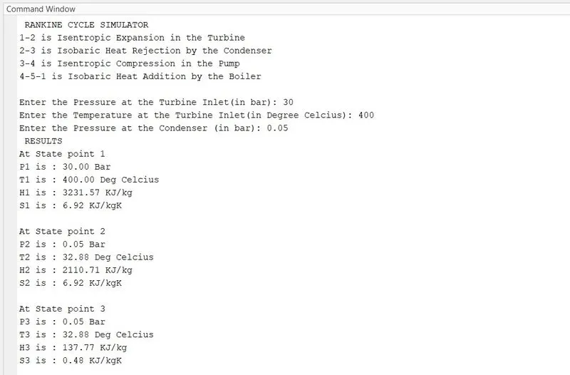
• Turbine Inlet Pressure = 30 bars
• Turbine Inlet temperature = 400° C
• Turbine Outlet Pressure = 0.05 bars = Condenser Inlet Pressure

2. The Program begins with clear all, close all, clc to erase the workspace and plots.
3. Input variables P1,T1,P2 are given by input command whose values are entered in command window while executing the Program.
4. At State-1, Values for Enthalpy & Entropy are extracted as a function of Pressure & Temperature. h_pT, s_pT, hL_p, sV_p etc.. are the default variables whose value is stored in XSteam file.
5. Similarly, all the variables for all states (State 2, 3, 4 & 5) are extracted using a suitable format.
6. Finally Work done, Thermal Efficiency, Back work ratio and SSC are calculated by basic formulae.
7. To plot the Saturation Curve, a Temperature range is defined using linspace command and for the overall length of this Temperature values of Enthalpy and Entropy are calculated at every temperature point. Now all the necessary data is found out, Plotting is done for both T-S & H-S curves using the plot commands. Annotations are assigned using text command. Results of the Cycle Simulation is displayed over Comand window using fprintf command.

CONCLUSION:

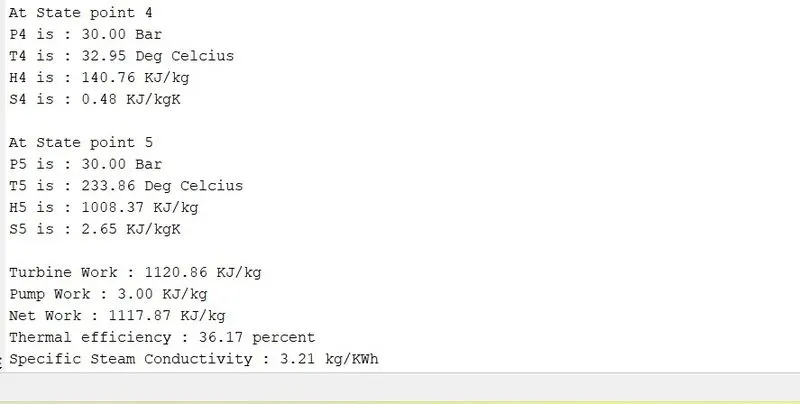
1. The values of all salient point’s Pressure, Temperature, Enthalphy and Entropy for different state points and also the Work, Efficiency, Back work ratio and Specific steam conductivity was calculated.
2. The graph of T-S and H-S for Rankine Cycle was plotted.