Week 4.1 - Genetic Algorithm

function [f] = Stalagmite(input_vector)

 x = input_vector(1);
 y = input_vector(2);
 f1_x = (sin(5.1*pi*x + 0.5)).^6;
 f1_y = (sin(5.1*pi*y + 0.5)).^6;
 t1 = ((x-0.0667).^2)/(0.64);
 f2_x = exp(-4.*log(2)*t1);
 t2 = ((y-0.0667).^2)/(0.64);
 f2_y = exp(-4.*log(2)*t2);
 f = -(f1_x.*f2_x.*f1_y.*f2_y);

end

The above code is derived in the stalagmite function in MATLAB using below formula.

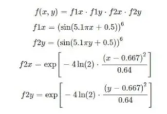
here the Negative sign shows that inverse of the Stalagmite function and is added in order to find the
Maximum value, as ga always gives the Minimum value.

Main Code

clear all
close all
clc

%% Search Space of the Function
 x=linspace(0,0.6,150);
 y=linspace(0,0.6,150);
 [X,Y]=meshgrid(x,y);

 num_cases=50; %Number of itreation for which the function will evaluate the fitness
 
%% Creating suface plot of stalagmite function

 for i=1:length(X)
 for j=1:length(Y)
 input_vector(1)=X(i,j);
 input_vector(2)=Y(i,j);
 f(i,j)=Stalagmite(input_vector); %values of function in given search space
 end
 end
 surfc(X,Y,-f); %generating the surface
 shading interp %To remove the lines produced by the mesh grid



 %% Iteration 1 - Statistical Behavious (Unbounded)

tic %calculating the study time through tic and toc command
for i=1:num_cases

 [inputs,fopt(i)]=ga(@Stalagmite,2); %calculating the optimized value of the function
 xopt(i)=inputs(1); %at each iteration
 yopt(i)=inputs(2);

end
study1_time=toc %displaying the time taken to evaluate


 % PLOTING THE GRAPH
 figure(1)
 subplot(2,1,1)
 surfc(X,Y,-f);
 hold on
 shading interp
 plot3(xopt,yopt,-fopt,'marker','o','markersize',5,'markerfacecolor','r');
 xlabel('x');
 ylabel('y');
 grid on
 subplot(2,1,2)
 plot(-fopt);
 xlabel('iterations')
 ylabel('function min value')

 %% Iteration 2 - Statistical Behavious (Bounded)

tic %calculating the study time through tic and toc command
 for j=1:num_cases

 [inputs,fopt(j)]=ga(@Stalagmite,2,[],[],[],[],[0;0],[1;1]); %calculating the optimized value of the function

xopt(j)=inputs(1); %at each iteration with boundation
 yopt(j)=inputs(2);

 end
study2_time=toc

 %PLOTTING
 figure(2)

 subplot(2,1,1)
 hold on
 surfc(X,Y,-f)
 shading interp
 plot3(xopt,yopt,-fopt,'marker','o','markersize',5,'markerfacecolor','r');
 xlabel('x');
 ylabel('y');
 grid on
 subplot(2,1,2)
 plot(-fopt);
 xlabel('iterations')
 ylabel('function min value')

%% Iteration 3 - Modifying Size of Population 

 options=optimoptions('ga','populationsize',300) %increaing the size of population by using
 %optimizations function

 tic
for k=1:num_cases

 [inputs,fopt(k)]=ga(@Stalagmite,2,[],[],[],[],[0;0],[1;1],[],[],options);
 xopt(k)=inputs(1);
 yopt(k)=inputs(2);

end
study3_time=toc

 %PLOTTING
 figure(3)

 subplot(2,1,1)
 hold on
 surfc(X,Y,-f)
 shading interp
 plot3(xopt,yopt,-fopt,'marker','o','markersize',5,'markerfacecolor','r');
 xlabel('x');
 ylabel('y');
 grid on
 subplot(2,1,2)
 plot(-fopt);
 xlabel('iterations')
 ylabel('function min value')

Explanation on main function used in Code

tic ---- calculating the study time through tic and toc command (Start Time of the code)