Week 4.1 - Genetic Algorithm

MATLAB Code to optimize the stalagmite function and find the global maxima of the function. I have started the code with basic commands clear all, close all, clc. Then defined the search space using linspace command created 2d arrays (X, Y) with 150 values between 0 to 0.6. In below-provided code also mentioned some necessary comments, created another Stalgmite function used in the main code did 3 studies to evaluate the maxima (Desired Output).

MAIN Code-

clear all
close all
clc

% Defining Our Search Space

x=linspace(0,0.6,150);
y=linspace(0,0.6,150);
num_cases=50 % No. of Iteration

% Creating 2-Dim Mesh
[xx yy]= meshgrid(x,y);

% Evaluating the Stalgmite function 
for i= 1:length(xx)
    for j= 1:length(yy)
        input_vector(1)=xx(i,j);
        input_vector(2)=yy(i,j);
        f(i,j)=stalgmite_fun(input_vector); % calling Created Function
    end
end

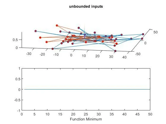
% Study-1 |Statistical Behaviour|In Unounded Conditions
tic % Calculating command for iterations
for i=1:num_cases
    [inputs,fopt(i)]=ga(@stalgmite_fun, 2);
    xopt(i)=inputs(1);
    yopt(i)=inputs(2);
end


study1_time=toc

% Graph Plotting

figure(1)
subplot(2,1,1)
hold on
surfc(x,y,f)
shading interp
plot3(xopt,yopt,fopt,'marker','o','MarkerSize',5,'MarkerFaceColor','r')
title('unbounded inputs')
subplot(2,1,2)
plot(fopt)
xlabel('iterations')
xlabel('Function Minimum')

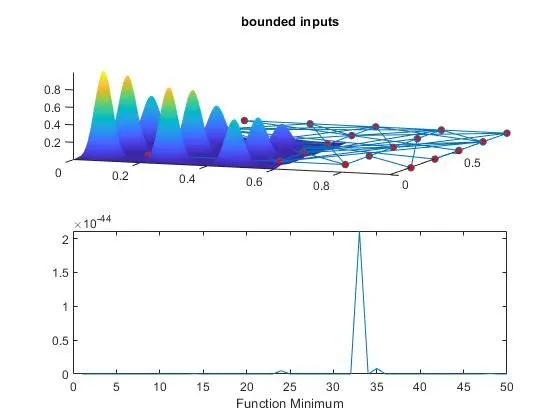
% Study-2 |Statistical Behaviour with- upper & Lower Bounds
tic
for i=1:num_cases
  [inputs,fopt(i)]=ga(@stalgmite_fun,2,[],[],[],[],[0,0],[1,1]);
    xopt(i)=inputs(1);
    yopt(i)=inputs(2);
end
study_2_time= toc

% Graph Plotting
figure(2)
subplot(2,1,1)
hold on
surfc(x,y,f)
shading interp
plot3(xopt,yopt,fopt,'marker','o','MarkerSize',5,'MarkerFaceColor','r')
title('bounded inputs')
subplot(2,1,2)
plot(fopt)
xlabel('iterations')
xlabel('Function Minimum')

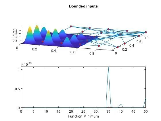
% Study-3 Increasing GA Iterations
options=optimoptions('ga')                         % Calculating the optimum solutions for Increasing the size of Population
options=optimoptions(options,'PopulationSize',240)

tic
for i=1:num_cases
    [inputs,fopt(i)]=ga(@stalgmite_fun,2,[],[],[],[],[0;0],[1;1],[],[],options);
    xopt(i)=inputs(1);
    yopt(i)=inputs(2);
end
study3_time=toc

figure(3)
subplot(2,1,1)
hold on
surfc(x,y,f)
shading interp
plot3(xopt,yopt,fopt,'marker','o','MarkerSize',5,'MarkerFaceColor','r')
title('Bounded inputs')
subplot(2,1,2)
plot(fopt)
xlabel('iterations')
xlabel('Function Minimum')

Results-

Study-1

Study-2 (UN-Bounded)

Study-3

Stalagmite Function Code-

function [f]= stalgmite_fun(input_vector)
f1x= (sin((5.1*pi).*input_vector(1)+0.5)).^6;
f1y= (sin((5.1*pi).*input_vector(2)+0.5)).^6;

f2x= exp((((input_vector(1)-0.0667).^2)/0.64).*(-4*log(2)));
f2y= exp((((input_vector(2)-0.0667).^2)/0.64).*(-4*log(2)));
f1=f1x*f1y*f2x*f2y;
f=f1;
end

GA- A genetic algorithm (GA) is a method for solving both constrained and unconstrained optimization problems based on a natural selection process that mimics biological evolution.

Genetic algorithms are a class of numerical and combinational optimizers which are especially useful for solving complex nonlinear and nonconvex problems.