Project 2 - Rankine cycle Simulator

• Rankine cycle Simulator MATLAB Code-
• Program initially started with the displays the process involved in Rankine cycle
• State 1& 2 of pressure (Inlet and outlet) and inlet of temperature are taken as an inputs
• The values from XStream Liberary are extracted and state values such as temp, pressure, enthalpy and entropy are calculated
• Note:- Xtream function code should be in the current directory otherwise it will not showing the results in the form of output.
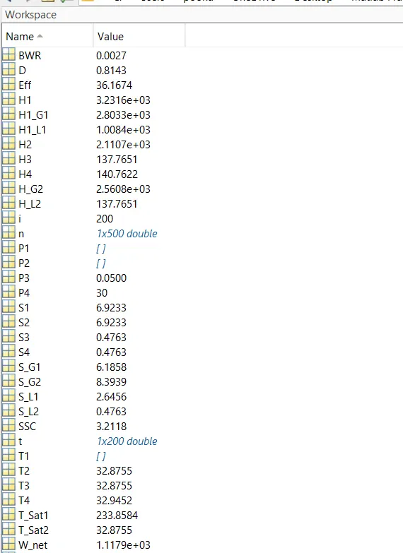
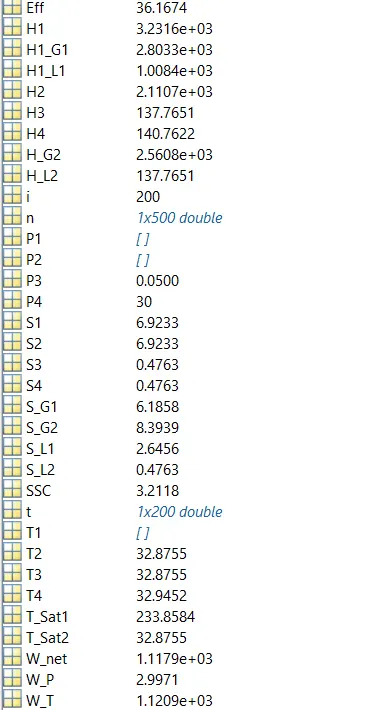
• Further the values of turbine work, pump work, net work, thermal eff, back ratio and specific steam conductivity are calculated
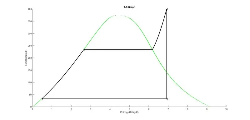
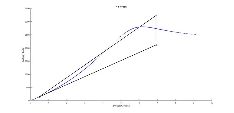
• Finally the T-S and H-S graph of the cycle is plotted through the code.

Code-

Clear all
Close all
clc
disp('   Rankine Cycle Simulator  ');
disp('1-2 is isentropic Expansion in the Turbine');
disp('2-3 is Constant Pressure heat Rejection by the Condensor');
disp('3-4 is isentropic Compression in the Pump');
disp('4-1 is Constant Pressure heat Addition by the Boiler');
fprintf('n')

% Taking Inputs 
P1= input('Enter the pressure at the turbine Inlet(in Bar):30 ');
T1= input('Enter the temperature at the Turbine inlet (in Degree Celcius):400 ');
P2= input('Enter the pressure at the condensor(in Bar):0.05');

% Calculating State Values

%At State point 1

H1= XSteam('h_pt',30,400);
S1= XSteam('s_pt',30,400);
H1_L1= XSteam('hL_p',30);
H1_G1= XSteam('hV_p',30);
S_L1= XSteam('sL_p',30);
S_G1= XSteam('sV_p',30);
T_Sat1= XSteam('Tsat_p',30);

%At State point 2
S2=S1;
S_L2= XSteam('sL_p',0.05);
S_G2= XSteam('sV_p',0.05);
D=(S2-S_L2)/(S_G2-S_L2); % Calculating the Dryness Fraction
H_L2= XSteam('hL_p',0.05);
H_G2= XSteam('hV_p',0.05);
H2= H_L2+D*(H_G2-H_L2); % Calculating the enthaply at point 2
T2= XSteam('T_ph',0.05,2.110708212003693e+03)
T_Sat2= XSteam('Tsat_p',0.05);

%At State point 3
P3=0.05;% P3= P2
T3=32.875489523760166; % T3=T2
H3=1.377651189884906e+02; %H3=H_L2
S3=0.476253789505102; %S3=S_L2

%At State point 4
P4=30; % P4= P3
S4=S3; % S4=S3
T4=XSteam('T_ps',P4,S4);
H4=XSteam('H_ps',P4,S4);

% Calculating Work ratio, Back work ratio,Specific Steam Conductivity and
% Efficiency

% Turbine Work
W_T=H1-H2;

% Pump Work
W_P= H4-H3;

% Net Work
W_net= W_T-W_P;

% Thermal Efficiency of the Rankine Cycle
Eff= (W_net/(H1-H4))*100;

% Back work ratio
BWR= W_P/W_T;

% Specific Steam Conductivity
SSC= 3600/W_T;

% Display Results
% State Point 1
disp('   Results     ');
disp('at state point 1');
fprintf('np1 is : %.2f bar n',P1);
fprintf('T1 is : %.2f Deg celcius n',T1);
fprintf('H1 is : %.2f KJ/kg n',H1);
fprintf('S1 is : %.2f KJ/kgK nn',S1);

% Values at State point 2
disp('at state point 2');
fprintf('np2 is : %.2f bar n',P2);
fprintf('T2 is : %.2f Deg celcius n',T2);
fprintf('H2 is : %.2f KJ/kg n',H2);
fprintf('S2 is : %.2f KJ/kgK nn',S2);


% Values at State point 3
disp('at state point 3');
fprintf('np3 is : %.2f bar n',P3);
fprintf('T3 is : %.2f Deg celcius n',T3);
fprintf('H3 is : %.2f KJ/kg n',H3);
fprintf('S3 is : %.2f KJ/kgK nn',S3);

% Values at State point 4
disp('at state point 4');
fprintf('np4 is : %.2f bar n',P4);
fprintf('T4 is : %.2f Deg celcius n',T4);
fprintf('H4 is : %.2f KJ/kg n',H4);
fprintf('S4 is : %.2f KJ/kgK nn',S4);

% Turbine Work
fprintf('nTurbine Work :%.2f KJ/kg n',W_T);

% Pump Work
fprintf('Pump Work :%.2f KJ/kg n',W_P);

% NET Work
fprintf('Net Work :%.2f KJ/kg n',W_net);

% Turmal Efficiency
fprintf('thermal efficiency :%.2f %',Eff);

% Specific Steam Conductivity
fprintf('nSpecific Steam Conductivity :%.2f KJ/kWh n',SSC);

% Back Work Ratio
fprintf('Back Work Ratio is : %f n',BWR);

% Plotting of T-S Curve
t= linspace(0,373.5,200);
figure(1)
hold on

for i=1:length(t)
    plot(XSteam('sL_T',t(i)),t(i),'g.')
    plot(XSteam('sV_T',t(i)),t(i),'g.')
end

plot([S1,S2],[T1,T2],'linewidth',2,'color','k')
text(S1,T1,'1','fontsize',10)
if D>1
T3= T_Sat2;
plot([S2,S_G2 S3 S4],[T2,T_sat2 T3 T4],'linewidth',2,'color','k')
T2 =T_Sat2;
text(S2,T2,'2','fontsize',10)
text(S3,T3,'3','fontsize',10)
else
plot([S2 S3 S4],[T2 T3 T4],'linewidth',2,'color','k')  
text(S2,T2,'2','fontsize',10)
text(S3,T3,'3','fontsize',10)
end

n= linspace(T1,T2,500);
for i= 1:length(n)
plot(XSteam('s_pT',P1,n(i)),n(i),'.','linewidth',2,'color','k')
end

plot([S_L1,S_G1],[T_Sat1 T_Sat1],'linewidth',2,'color','k')
text (S_L1,T_Sat1,'4','fontsize',10)
xlabel('Entropy(KJ/kg-K)')
ylabel('Temperature(k)')
title('T-S Graph')

% Plotting of H-S Curve

figure(2)
hold on
for i=1:length(t)
    plot(XSteam('sL_T',t(i)),XSteam('hL_T',t(i)),'b.')
    plot(XSteam('sV_T',t(i)),XSteam('hV_T',t(i)),'b.')
end
plot([S1 S2 S3 S4 S1],[H1 H2 H3 H4 H1],'linewidth',2,'color','k')  
text(S1,H1,'1','fontsize',10)
text(S2,H2,'2','fontsize',10)
text(S3,H3,'3','fontsize',10)
text(S4,H4,'4','fontsize',10)
xlabel('Entropy(KJ/kg-K)')
ylabel('Enthalpy(kJ/kg)')
title('H-S Graph')

output values window-

Graph Plotting Images- T-S Graph

H-S Graph-

During the programing part many error faced many of them were Spell mistakes or somewhere i have used caps alphabets and some where i used the same with lower caps so the error pops ups that matlab doesn't recorgnise this (X-Y-z) Function.

So make sure you have used the particular function with the same varibale or name.