Week 4.1 - Genetic Algorithm
Aim
Try to understand the concept of genetic algorithm by referring to varius sources before you attend this challenge. Look out for information regarding stalagmite function and ways to optimise it.
Write a code in MATLAB to optimise the stalagmite function and find the global maxima of the function.
Clearly expalin the concept of genetic algorithm in your own words and also explain the syntax for ga in MATLAB in your report.
Make sure that your code gives the same output, even if it is made to run several times.
Plot graphs for all 3 studies and for F maximum vs no. of iterations. Title and axes labels are a must, legends could be shown if necessary.
- Stalagmite Function is a function to determine global min and global max. By that we can get lot of things like mainly its use to genrate the population in future years. Stalagmite structures are formed from the cave floor that point upward.
- The below format is the structure to get the global max and min.
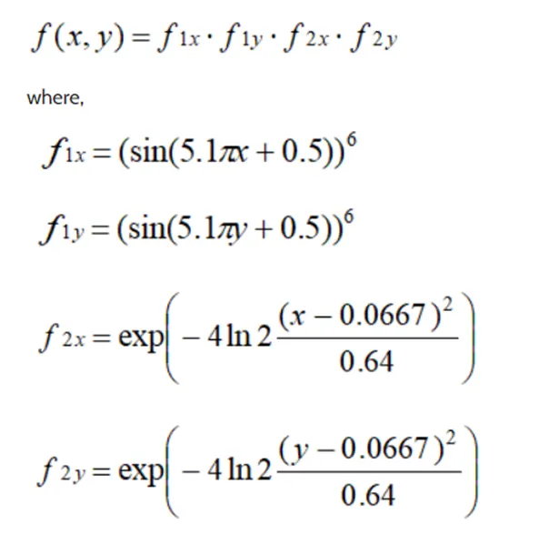
The stalagmite function is defined as below mentioned equation
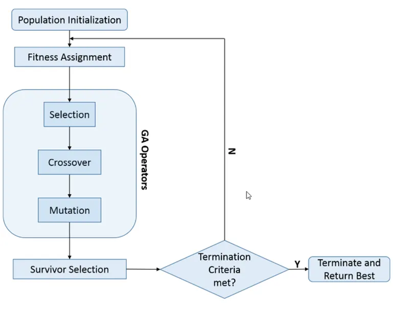
- The below syntaxes have been used to solve the ga function
1 . x = ga(fun,nvars) finds a local unconstrained minimum, x, to the objective function, fun. nvars is the dimension (number of design variables) of fun.
- x = ga(fun,nvars,A,b,Aeq,beq,lb,ub) defines a set of lower and upper bounds on the design variables, x, so that a solution is found in the range lb ≤ x ≤ ub. (Set Aeq=[] and beq=[] if no linear equalities exist.)
- x = ga(fun,nvars,A,b,Aeq,beq,lb,ub,nonlcon,options) minimizes with the default optimization parameters replaced by values in options. (Set nonlcon=[] if no nonlinear constraints exist.) Create options using optimoptions.
%Function code used in the code
function[F]=stalagmite_func(input_vector)
a=input_vector(1);
b=input_vector(2);
f1_x=[sin(5.1*pi*a+0.5)]^6;
f1_y=[sin(5.1*pi*b+0.5)]^6;
f2_x=exp(-4*log(2)*((a-0.0667)^2/0.64));
f2_y=exp(-4*log(2)*((b-0.0667)^2/0.64));
F=f1_x*f1_y*f2_x*f2_y;
F=-F; %to find the maximum value we change the sign of function
end
% MATLAB code is used to run the function
% for the study case 1 x = ga(fun,nvars)
clear all
close all
clc
%inputs
x=linspace(0,0.5,180);
y=linspace(0,0.5,180);
%creating a 2D mesh
[xx,yy]=meshgrid(x,y);
% function_output = get_stalagmite(xx,yy)
for i=1:length(xx) %xx is derived like using linspace
for j=1:length(yy) %yy is derived like using linspace
input_vector(1)=xx(i,j);
input_vector(2)=yy(i,j);
F(i,j)=stalagmite_func(input_vector);
end
end
%to plot a surface graph
surf(xx,yy,- F) %creating a 3D surface plot for the stalagmite function with a countor plot.
colorbar
xlabel('x_values');
ylabel('y_values');
zlabel('F_values');
shading interp %shading coomond use to remove the grids lines
axis tight
%study case 1
num_case =50;
tic
for i=1:num_case;
[input,output(i)]=ga(@stalagmite_func,2);
xopt(i)=input(1)
yopt(i)=input(2)
end
time=toc
figure(1)
subplot(2,1,1)
surf(xx,yy,- F) %creating a 3D surface plot for the stalagmite function with a countor plot.
colorbar
xlabel('x_values');
ylabel('y_values');
zlabel('F_values');
shading interp %shading coomond use to remove the grids lines
hold on
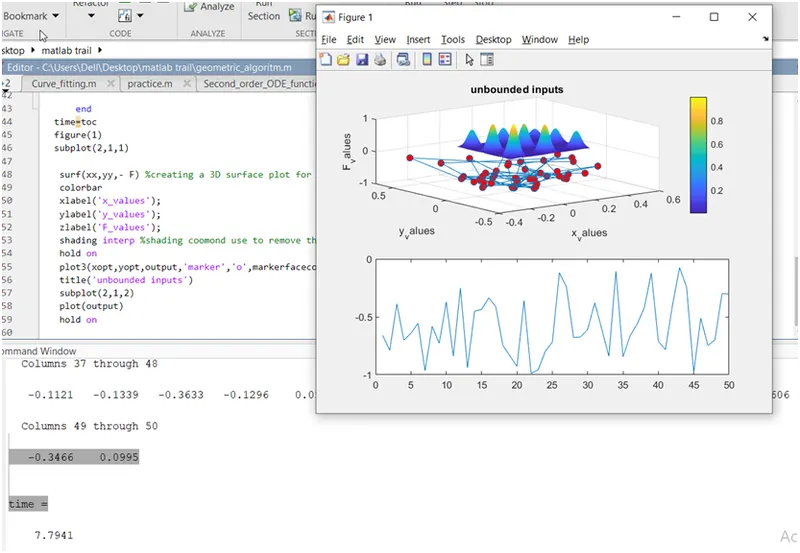
plot3(xopt,yopt,output,'marker','o',markerfacecolor='r')
title('unbounded inputs')
subplot(2,1,2)
plot(output)
hold on
% for the study case 2 x = ga(fun,nvars,A,b,Aeq,beq,lb,ub)
clear all % clear the workspace
close all % clear all the figure window
clc % clear the command window
%inputs
x=linspace(0,0.5,180);
y=linspace(0,0.5,180);
%creating a 2D mesh
[xx,yy]=meshgrid(x,y);
% function_output = get_stalagmite(xx,yy)
for i=1:length(xx) %xx is derived like using linspace
for j=1:length(yy) %yy is derived like using linspace
input_vector(1)=xx(i,j);
input_vector(2)=yy(i,j);
F(i,j)=stalagmite_func(input_vector);
end
end
%to plot a surface graph
surf(xx,yy,- F) %creating a 3D surface plot for the stalagmite function with a countor plot.
colorbar
xlabel('x_values');
ylabel('y_values');
zlabel('F_values');
shading interp %shading coomond use to remove the grids lines
axis tight
%study case 2
num_case =50;
tic
for i=1:num_case;
[input,output(i)]=ga(@stalagmite_func,2,[],[],[],[],[0,0],[0.5,0.5]);
xopt(i)=input(1)
yopt(i)=input(2)
end
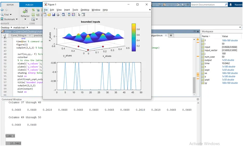
time=toc % command use to note the tome of function
figure(1)
subplot(2,1,1) % Subplot command is used to plot many images in one as per that syntax subplot(row.coloum,image)
surf(xx,yy,- F) %creating a 3D surface plot for the stalagmite function with a countor plot.
colorbar
% to show the lables
xlabel('x_values');
ylabel('y_values');
zlabel('F_values');
shading interp %shading coomond use to remove the grids lines
hold on
plot3(xopt,yopt,output,'marker','o',markerfacecolor='r')
title('unbounded inputs')
subplot(2,1,2)
plot(output)
hold on
% for the study case 3 x = ga(fun,nvars,A,b,Aeq,beq,lb,ub,nonlcon,options)
clear all % clear the workspace
close all % clear all the figure window
clc % clear the command window
%inputs
x=linspace(0,0.5,180);
y=linspace(0,0.5,180);
%creating a 2D mesh
[xx,yy]=meshgrid(x,y);
% function_output = get_stalagmite(xx,yy)
for i=1:length(xx) %xx is derived like using linspace
for j=1:length(yy) %yy is derived like using linspace
input_vector(1)=xx(i,j);
input_vector(2)=yy(i,j);
F(i,j)=stalagmite_func(input_vector);
end
end
%to plot a surface graph
surf(xx,yy,- F) %creating a 3D surface plot for the stalagmite function with a countor plot.
colorbar
xlabel('x_values');
ylabel('y_values');
zlabel('F_values');
shading interp %shading coomond use to remove the grids lines
axis tight
%study case 3
num_case =50;
options=optimoptions("ga")
options=optimoptions(options,'PopulationSize',300);
tic
for i=1:num_case;
[input,output(i)]=ga(@stalagmite_func,2,[],[],[],[],[0,0],[0.5,0.5],[],options);
xopt(i)=input(1)
yopt(i)=input(2)
end
time=toc % command use to note the tome of function
figure(1)
subplot(2,1,1) % Subplot command is used to plot many images in one as per that syntax subplot(row.coloum,image)
surf(xx,yy,- F) %creating a 3D surface plot for the stalagmite function with a countor plot.
colorbar
% to show the lables
xlabel('x_values');
ylabel('y_values');
zlabel('F_values');
shading interp %shading coomond use to remove the grids lines
hold on
plot3(xopt,yopt,output,'marker','o',markerfacecolor='r')
title('bounded inputs')
subplot(2,1,2)
plot(output)
hold on
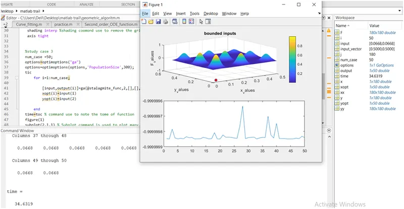
Errors while writting the code
- I have written a wrong variables by changing them i got to overcome this error
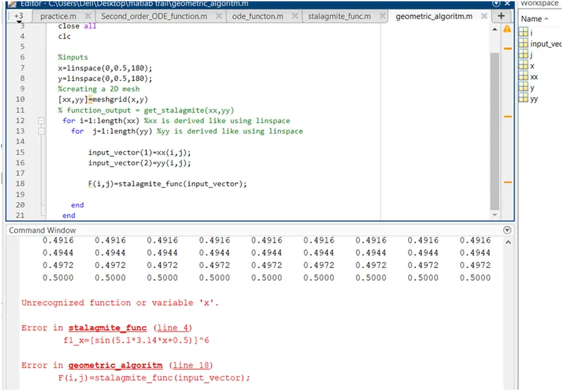
- By adding removing square brackets and adding of common brackets
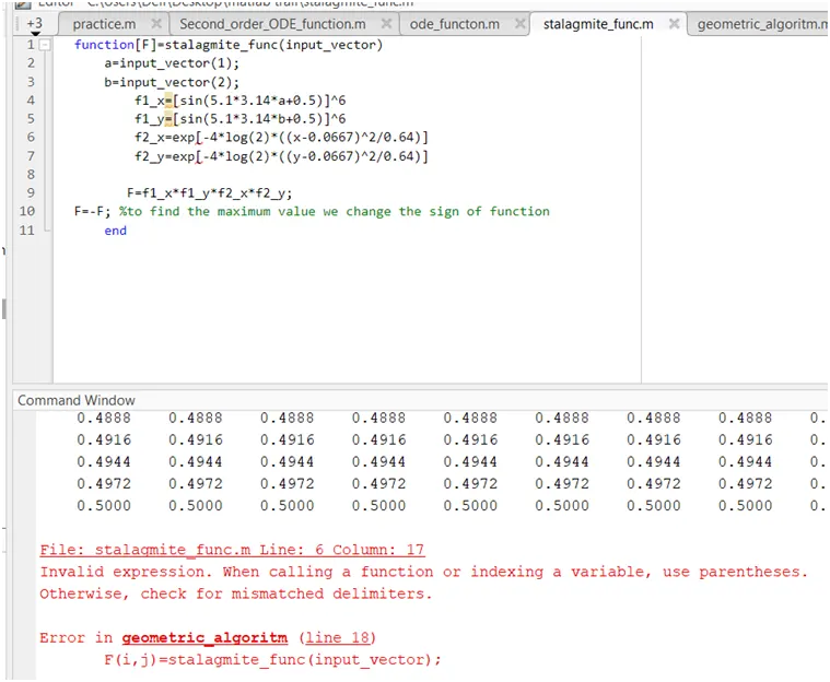
-
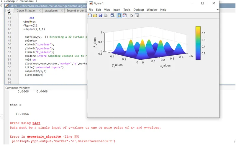
error of markerfacecolor