Week 4.1 - Genetic Algorithm
AIM: To study about genetic algorithm and to calculate the global maxima of stalagmite function using Genetic Algorithm in MATLAB.
Objective:-
- To study about Genetic Algorithm and stalagmite function.
- To write a code in matlab to optimise the stalagmite funtion and find the global maxima of the function.
- To plot graphs based on the studies done for Genetic Algorithm.
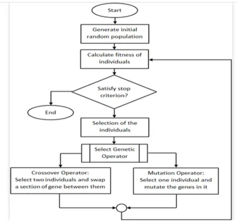
The basic steps in creating a genetic algorithm is as follows,
- The algorithm creates a random initial population at beginning.
- Then to create new population, the algorithm scores each member of the current population by computing its fitness value and converts them into a more usable range of values.
- Then based on these new values the algorithm selects members, called as parents.
- Then the algorithm produces children from the parents. Children are produced either by making random changes to a single parent which is mutation or by combining the vector entries of a pair of parents which is crossover.
- in this way the algorithm replaces the current population with the children to form the next generation.
- The algorithm stops when it reaches any one of the specified factors such as time limit, fitness limit, generations, function tolerance, constraint tolerance, etc.
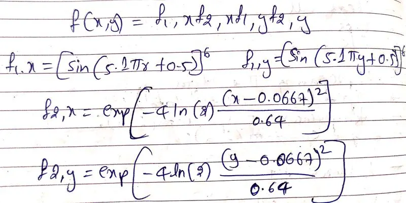
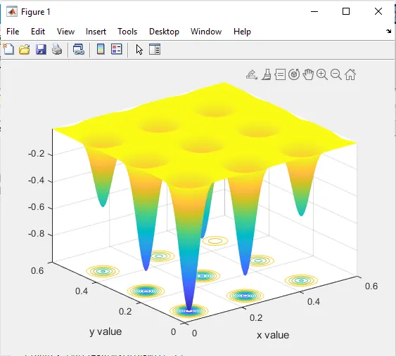
Stalagmite function:-
The flowchart for Genetic Algorithm is given below.
Coding :-
%program for a Genetic Algorithim
clear all
close all
clc
%defining our search space
x=linspace(0,0.6,150);
y=linspace(0,0.6,150);
[xx,yy]=meshgrid(x,y);
%Evaluating the stalagmite function
for i=1:length(x)
for j=1:length(y)
input_vector(1)=xx(i,j);
input_vector(2)=yy(i,j);
f(i,j)=stalagmite(input_vector);
end
end
surfc(xx,yy,f)
xlabel('x value')
ylabel('y value')
shading interp
[inputs,fval]=ga(@stalagmite,2)
CODE for stalagmite function:-
function[f]=stalagmite(input_vector)
%intializing x and y input
x=input_vector(1);
y=input_vector(2);
%term x1 is equation for f1_x and term y1 is equation for f1_y
termx1=(sin(5.1*pi*x+0.5))^6;
termy1=(sin(5.1*pi*y+0.5))^6;
%term x2 is the equation for f2_x and term y2 is the equation for f2_y
termx2=exp(-4*log(2)*((x-0.0667)^2/0.64));
termy2=exp(-4*log(2)*((y-0.0667)^2/0.64));
f=-termx1*termy1*termx2*termy2;
end
Output:-
STUDY 1:-
%program for a Genetic Algorithim
clear all
close all
clc
%defining our search space
x=linspace(0,0.6,150);
y=linspace(0,0.6,150);
[xx,yy]=meshgrid(x,y);
%Evaluating the stalagmite function
for i=1:length(x)
for j=1:length(y)
input_vector(1)=xx(i,j);
input_vector(2)=yy(i,j);
f(i,j)=stalagmite(input_vector);
end
end
num_case=150
tic
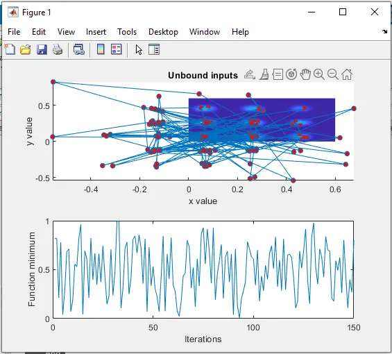
%Study 1- statistical behaviour
for i=1:num_case
[inputs,fopt(i)]=ga(@stalagmite,2);
xopt(i)=inputs(1);
yopt(i)=inputs(2);
end
study1_time=toc
figure(1)
subplot(2,1,1)
hold on
surfc(x,y,-f)
xlabel('x value')
ylabel('y value')
shading interp
plot3(xopt,yopt,-fopt,'marker','o','markersize',5,'markerfacecolor','r')
title('Unbound inputs')
subplot(2,1,2)
plot(-fopt)
xlabel('Iterations')
ylabel('Function minimum').
Output:-
STUDY2:-
clear all
close all
clc
%defining our search space
x=linspace(0,0.6,150);
y=linspace(0,0.6,150);
num_case=50;
%creating a 2Dimensional mesh
[xx,yy]=meshgrid(x,y);
%evaluating the stalagmite function
for i=1:length(xx)
for j=1:length(yy)
input_vector(1)=xx(i,j);
input_vector(2)=yy(i,j);
f(i,j)=stalagmite(input_vector);
end
end
%study 2 for the optimization
for i=1:num_case
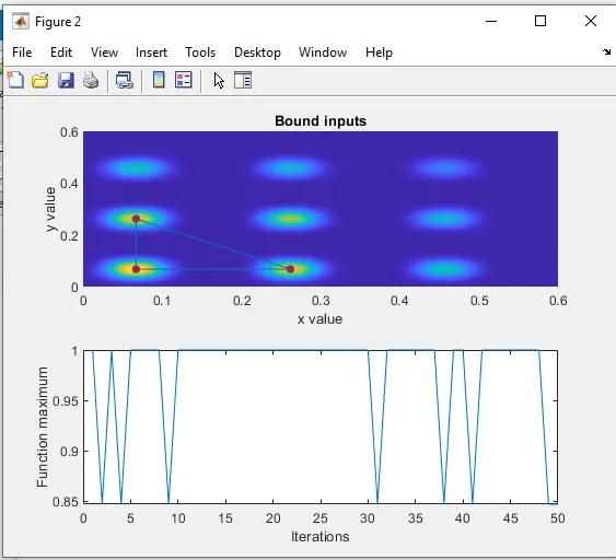
[inputs,fopt(i)]=ga(@stalagmite,2,[],[],[],[],[0,0],[0.5,0.5]);
xopt(i)=inputs(1);
yopt(i)=inputs(2);
end
figure(2)
subplot(2,1,1)
hold on
surfc(x,y,-f)
xlabel('x value')
ylabel('y value')
shading interp
plot3(xopt,yopt,-fopt,'marker','o','markersize',5,'markerfacecolor','r')
title('Bound inputs')
subplot(2,1,2)
plot(-fopt)
xlabel('Iterations')
ylabel('Function maximum')
Output:-
STUDY 3:-
clear all
close all
clc
%defining our search space
x=linspace(0,0.6,150);
y=linspace(0,0.6,150);
num_case=50;
%creating a 2Dimentional mesh
[xx,yy]=meshgrid(x,y);
%Evaluating the stalagmite function
for i=1:length(xx)
for j=1:length(yy)
input_vector(1)=xx(i,j);
input_vector(2)=yy(i,j);
f(i,j)=stalagmite(input_vector);
end
end
options=optimoptions('ga')
options=optimoptions(options,'populationsize',360);
%study 2 for the optimization
for i=1:num_case
[inputs,fopt(i)]=ga(@stalagmite,2,[],[],[],[],[0;0],[0.5:0.5],[],[],options);
xopt(i)=inputs(1);
yopt(i)=inputs(2);
end
study2_time=toc
figure(2)
subplot(2,1,1)
hold on
surfc(x,y,-f)
xlabel('x value')
ylabel('y value')
shading interp
plot3(xopt,yopt,-fopt,'marker','o','markersize',5,'markerfacecolor','r')
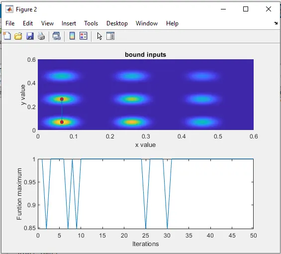
title('bound inputs')
subplot(2,1,2)
plot(-fopt)
xlabel('Iterations')
ylabel('Funtion maximum')
Output:-
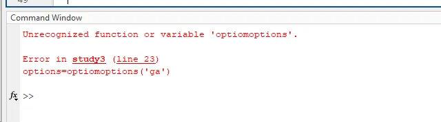
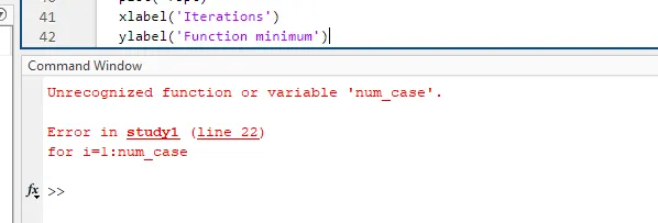
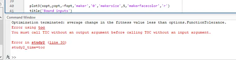
Errors occured during coding:-