Week 3 - Solving second order ODEs
Aim: To solve an ordinary differential equation (ODE) and use the calculated information to animate the motion of the pendulum via Matlab.
Introduction:
Pendulums have many applications and were utilized often before the digital age. They are used in clocks and metronomes due to the regularity of their period , in wrecking balls and playground swings, due to their simple way of building up and keeping energy.
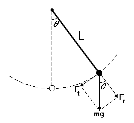
The figure at the right shows an idealized pendulum, with a massless string or rod of length L and bob of mass m . The open circle shows the rest position of the bob. when the bob is moved from its rest position and let go , it swings back and forth.The time it takes the pendulum to swing from its farthest right position to its farthest left position and back to its next farthest right position is the period of the pendulum.
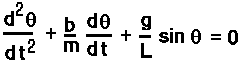
An ordinary differential equation is a differential equation containing one or more function of one independent variable and the derivatives of those funtions.The ODE equation and the calculation are shown below.
Code Explanation:-
%solving second order ODEs of a pendulum
clear all
close all
clc
%given data
b= 0.05
g= 9.81
l= 1
m= 0.1
%initial condition
%angular displacement is 0 and angular velocity is 5
theta_0 = [0;5]
%time span
%pendulum oscillates between 0-20 seconds
t_span = linspace(0,20,500)
%solve ODE
[t,results]=ode45(@(t,theta) ode_func(t,theta,b,g,l,m),t_span,theta_0);
%plotting
plot(t,results(:,1))
hold on
plot(t,results(:,2))
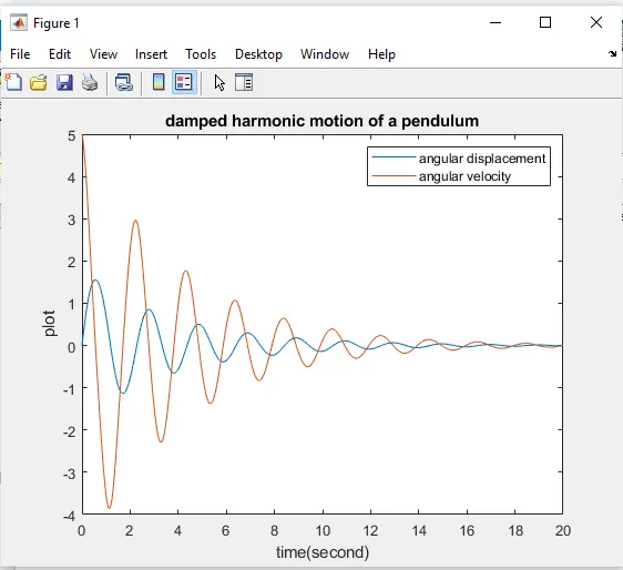
title('damped harmonic motion of a pendulum')
legend('angular displacement','angular velocity')
xlabel('time(second)')
ylabel('plot')
%for loop
%before starting the for loop, a counter value was defined
ct=1;
for i=1:length(results(:,1))
x_start = 0
y_start = 0
x_end = 1*sin(results(i,1))
y_end = -1*cos(results(i,1))
%plotting the animation
plot([-1 1],[0 0],'linewidth',5)
hold on
plot([x_start x_end],[y_start y_end],'linewidth',3)
hold on
plot(x_end,y_end,'0','markersize',20)
title('animation of transient behaviour of a pendulum')
axis([-1.5 1.5 -1.5 1])
pause(0.03)
hold off
m(ct)= getframe(gcf)
ct =ct+1
end
%animation of the pendulum
movie(M)
videofile=VideoWriter('pendulum animation.avi','uncompressed avi')
open(videofile)
writevideo(videofile,M)
close(videofile)
functioning:
%ODE
function[dtheta_dt]= ode_func(t,theta,b,g,l,m)
theta1=theta(1)
theta2=theta(2)
dtheta1_dt=theta2
dtheta2_dt=-(b/m)*theta2-(g/l)*sin(theta1)
dtheta_dt=[dtheta1_dt;dtheta2_dt]
end
The second part of the code is to establish a for loop, A for loop is a repetition control structure that allows you to efficiently write a loop that needs to erecute a specific number of times.
The final step of the code is to create a movie of the animation of the robotic arm ,so the movie command was used. The videowriter command was used to assign the video format,for this project.avi was used as the format.the open command was used to open the video. writevideo command was used to write the video with plot frames. finally the close command was used to close the video file.
Conclusion:-
The x_start,y_start , x_end, y_end values are shown below.
x_start =
0
y_start =
0
x_end =
0
y_end =
0
Animation video:-
https://drive.google.com/file/d/1RtDMKkQYxhbcvh-w32bstB10Tn_XDGZN/view?usp=sharing
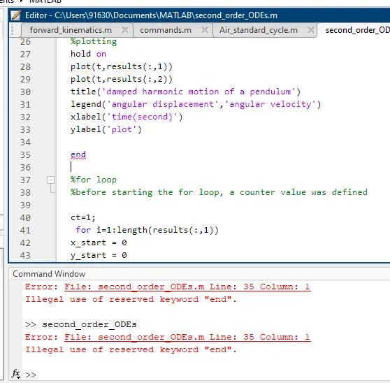
Errors found programing: