Week 4.1 - Genetic Algorithm

x = ga(fun,nvars) finds a local unconstrained minimum, x, to the objective function, fun. nvars is the dimension (number of design variables) of fun.

x = ga(fun,nvars,A,b,Aeq,beq,lb,ub) defines a set of lower and upper bounds on the design variables, x, so that a solution is found in the range lb ≤ x ≤ ub. (Set Aeq=[] and beq=[] if no linear equalities exist.)

x = ga(fun,nvars,A,b,Aeq,beq,lb,ub,nonlcon) subjects the minimization to the constraints defined in nonlcon. The function nonlcon accepts x and returns vectors C and Ceq, representing the nonlinear inequalities and equalities respectively. ga minimizes the fun such that C(x) ≤ 0 and Ceq(x) = 0. (Set lb=[] and ub=[] if no bounds exist.)

x = ga(fun,nvars,A,b,Aeq,beq,lb,ub,nonlcon,options) minimizes with the default optimization parameters replaced by values in options. (Set nonlcon=[] if no nonlinear constraints exist.) Create options using optimoptions.

x = ga(fun,nvars,A,b,Aeq,beq,lb,ub,nonlcon,intcon) or x = ga(fun,nvars,A,b,Aeq,beq,lb,ub,nonlcon,intcon,options) requires that the variables listed in intcon take integer values.

[x,fval] = ga(___), for any previous input arguments, also returns fval, the value of the fitness function at x.

[x,fval,exitflag,output] = ga(___) also returns exitflag, an integer identifying the reason the algorithm terminated, and output, a structure that contains output from each generation and other information about the performance of the algorithm.

[x,fval,exitflag,output,population,scores] = ga(___) also returns a matrix population, whose rows are the final population, and a vector scores, the scores of the final population.

Governing Equation for the Following program: -

`f(x,y)=f_(1,x)f_(2,x)f_(1,y)f_(2,y)`

`f_(1,x) =[sin(5.1pix+0.5)]^6`

`f_(1,y) =[sin(5.1piy+0.5)]^6`

`f_(2,x)=exp[-4ln(2)*(x-0.0667)^2/0.64]`

`f_(2,y)=exp[-4ln(2)*(y-0.0667)^2/0.64]`

Program: -

Function program

function [f] = stalagmite(input_vector)

x = input_vector(1);
y = input_vector(2);

%function formulas for genetic algorithm
f1 = [sin(5.1.*pi.*x+0.5)].^6;
f2 = [sin(5.1.*pi.*y+0.5)].^6;
f3 = exp(-4*log(2)*((x-0.0667).^2)./0.64);
f4 = exp(-4*log(2)*((y-0.0667).^2)./0.64);
f = -(f1*f2*f3*f4);

end

Main program

clear all
close all
clc

%Defining Our search space
x = linspace(0,0.6,150);
y = linspace(0,0.6,150);
num_cases = 50; %NO of iterations

%Creating a 2Dimentional mesh
[xx yy] = meshgrid(x,y);

%Evaluating the stalagmite function
for i = 1:length(xx)
    for j = 1:length(yy)
        input_vector(1)=xx(i,j);
        input_vector(2)=yy(i,j);
        f(i,j) = stalagmite(input_vector);
    end
end


 %study 1 - unbound inputs
tic
 for i = 1:num_cases
     [inputs,fopt(i)] = ga(@stalagmite, 2);% Genetic algorithm syntax
     xopt(i) = inputs(1);
     yopt(i) = inputs(2);
 end

 study1_time = toc

%Assigning figure no to plot 
figure(1)
 subplot(2,1,1)%Subplot command for analysing data
 hold on
 surfc(x,y,-f)
 shading interp %to eliminate grid lines
 plot3(xopt,yopt,-fopt,'Marker','o','MarkerSize',8,'MarkerFaceColor','r')
 xlabel('X')
 ylabel('Y')
 title('Unbounded inputs')
 subplot(2,1,2)
 plot(-fopt)
 xlabel('Iteration')
 ylabel('Maximum value of function')

 tic
 %study 2 - Bound inputs

 for i = 1:num_cases
     [inputs,fopt(i)] = ga(@stalagmite,2,[],[],[],[],[0;0],[0.6;0.6]);% Genetic algorithm syntax
     xopt(i) = inputs(1);
     yopt(i) = inputs(2);
 end

 study2_time = toc

 figure(2)
 subplot(2,1,1)
 hold on
 surfc(x,y,-f)
 shading interp
 plot3(xopt,yopt,-fopt,'Marker','o','MarkerSize',9,'MarkerFaceColor','r')
 xlabel('X')
 ylabel('Y')
 title('Bounded inputs')
 subplot(2,1,2)
 plot(-fopt)
 xlabel('Iteration')
 ylabel('Maximum value of function')

 
 
 %study 3 - Bound inputs
options = optimoptions('ga');
options = optimoptions(options,'PopulationSize',300);
 
tic
for i = 1:num_cases
     [inputs,fopt(i)] = ga(@stalagmite,2,[],[],[],[],[0;0],[0.6;0.6],[],[],options);% Genetic algorithm syntax
     xopt(i) = inputs(1);
     yopt(i) = inputs(2);
 end
study3_time = toc

 figure(3)
 subplot(2,1,1)
 hold on
 surfc(x,y,-f)
 shading interp
 plot3(xopt,yopt,-fopt,'Marker','o','MarkerSize',9,'MarkerFaceColor','r')
 xlabel('X')
 ylabel('Y')
 title('Bounded inputs')
 subplot(2,1,2)
 plot(-fopt)
 xlabel('Iteration')
 ylabel('Maximum value of function')

Code explanation with results: -

1. To start the program with clear all which clears the workspace, close all which closes all the previous plots, and clc which clears the command window.

2. Setting up the search space for a given problem, by considering the variables x and y with the linspace command. As x,y both are one-dimensional arrays with the help of the meshgrid command we are converting them into two-dimensional arrays and variables are xx, yy.

3. We have created a separate function file for the given problem statement which is named stalagmite.m. In this function, we have used the formulas that we have discussed in the governing equations above. here we are going to use the negative(-) sign so as to calculate global maxima.

4. Now we going to specify the input vector that is xx and yy and they are used to give inputs to our function.

5. Now for the study purpose we are going to take 50 iterations of the program.

6. Now we going to track the time that each study is going to take. so for that, we are going to use the tic command which helps to start the stopwatch. Make sure that we going to introduce the tic command before the for loop for the study starts and once the for loop ends we are going to take the reading by using the toc command.

Study 1 (Unbounded inputs): -

1. In the study 50 iterations are going to run as specified in the program. In the loop, we are providing 'ga' syntax in which we are going to input the function that we have generated and no 2 indicates two variables.

2. Now we going to plot the results of study one. to start plotting with the subplot command in MATLAB. subplot(m,n,p) divides the current figure into an m-by-n grid and creates axes in the position specified by p. The first subplot is the first column of the first row, the second subplot is the second column of the first row, and so on. If axes exist in the specified position, then this command makes the axes the current axes.

3. We have used the surfc command to plot the stalagmite function. In the surfc command, while plotting we have used the negative(-) sign to f so that we will be able to analyze the global maxima correctly. Also, we are going to use this negative sign in the plot command. and below that, we used 'Shading interp' which helps us to hide the grid line on the surface plot that we have plotted.

4. With the help of the subplot command we have plotted the second graph in the same figure.

5. Now we are going to label both the axis with help of 'xlabel' and 'ylabel' commands.

Outputs of study one: -

Explanation: -

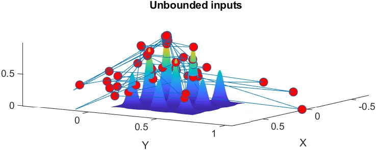
As we have mentioned in the procedure that we are going to use a negative sign to f while plotting the graph so that we will be able to Analyze the plot easily. So we aim to find the global maxima of the genetic algorithm. So the program did the random sampling and chose some values global maxima. but the graph looks shattered so we are going to bound the output so that we can find the proper output for the given program.

Explanation: -

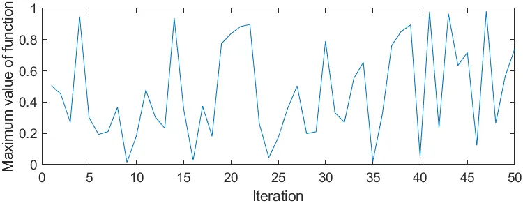
From the graph, we can see that we have got 50 different values for 50 iterations. We can see that value of the function is varying between 0 and 1. Now we have to bound the output so that we can get the precise value for global maxima. Which we are going to do in study 2. The time required to do study 1 is 3.1615.

Study 2 (Bounded inputs): -

The program for study 2 will be the same but we are going to modify the ga function. We are going to set upper and lower bounds so that a solution is found in the range between lb and ub. as we can see that we have introduced the lb and ub in the last part of syntax we can see that we have bounded them in 0 to 0.6 to x and y-axis.

As we have discussed in the syntax discussion we can see the explanation there.

x = ga(fun,nvars,A,b,Aeq,beq,lb,ub) defines a set of lower and upper bounds on the design variables, x so that a solution is found in the range lb ≤ x ≤ ub. (Set Aeq=[] and beq=[] if no linear equalities exist.)

[inputs,fopt(i)] = ga(@stalagmite,2,[],[],[],[],[0;0],[0.6;0.6])

Outputs for Study Two: -

Explanation: -

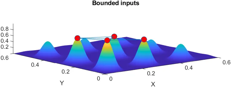
As we have discussed in the procedure we can be able to see that in the 3D plot which is a surface plot that our x and y-axis are bounded in 0 to 0.6. We can see that there are fewer points from random sampling with local and global maxima. We bounded the inputs that's why it's giving the precise value of global maxima.

Explanation: -

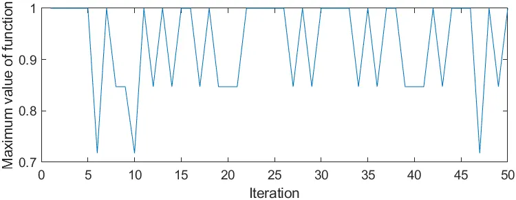
We can see as we have discussed earlier in the last result we can see that 50 different values of a function for 50 different iterations. But here we can see that some of the values of the function are similar to one another. and we can see that the 'Maximum value of function' is between 0.7 to 1 which is better than study one which shows that the output we have got is consistent. The time required to do study 2 is 3.8728.

Study 3(Bounded inputs): -

The program for study 3 will be the same but we are going to modify the ga function. Here in the third study, we have introduced options, which helps us to increase the population to increase the size. as we can see that we have introduced the lb and ub in the last part of syntax we can see that we have bounded them in 0 to 0.6 to x and y-axis. And after that, as discussed in syntax we are going to set noncolon. And after that, we going to introduce the option command that we have created.

As we can see below we have to introduce option command as shown below. Set options for ga by using optimoptions.

options = optimoptions('ga');

We are going to set the Population size to 300 as shown below.

options = optimoptions(options,'PopulationSize',300);

[inputs,fopt(i)] = ga(@stalagmite,2,[],[],[],[],[0;0],[0.6;0.6],[],[],options)

As we have discussed in the syntax discussion we can see the explanation there

x = ga(fun,nvars,A,b,Aeq,beq,lb,ub,nonlcon,options) minimizes with the default optimization parameters replaced by values in options. (Set nonlcon=[] if no nonlinear constraints exist.) Create options using optimoptions.

Outputs of study three: -

Explanation: -

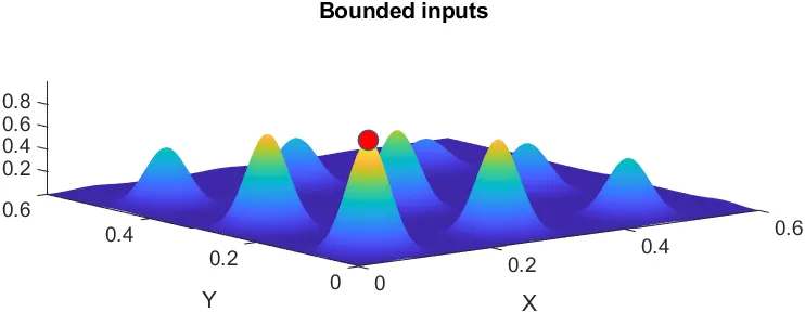
As we have discussed in the procedure we can be able to see that in the 3D plot which is a surface plot that our x and y-axis are bounded in 0 to 0.6. We can also see that we have got a single point for global maxima. We bounded the inputs and we have increased the population size to 300 that's why it's giving the precise value of global maxima. so it is giving nearly consistent value in the output which helps us to get precise value.

Explanation: -

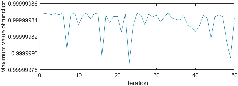
We can see as we have discussed earlier in the last result we can see that 50 different values of a function for 50 different iterations. But here we can see that most of the values of the function are similar to one another. and we can see that the 'Maximum value of function' is between 0.99999978 to 0.99999986 which is better than study two which shows that the output we have got is consistent. In that also we can see that most of the 'Maximum value of function' lies between 0.99999984 to 0.99999986 which result in getting one point of Global Maxima. The time required to do study 1 is 14.9219.