Week 4.1 - Genetic Algorithm

A genetic algorithm (GA) is a method for solving both constrained and unconstrained optimization problems based on a natural selection

process that mimics biological evolution.

The algorithm repeatedly modifies a population of individual solutions. At each step, the genetic algorithm randomly selects individuals

from the current population and uses them as parents to produce the children for the next generation. Over successive generations, the

population "evolves" toward an optimal solution.

We can apply the genetic algorithm to solve problems that are not well suited for standard optimization algorithms, including problems in

which the objective function is discontinuous,

non-differentiable, stochastic, or highly nonlinear.

By default, in MATLAB ga calculates the minimum value of a function. So to find the global maximum of a function we can invert the

function whose global maximum is to be found,find the minimum value of the inverted function, the negative of the minimum value will

give the global maximum of the function.

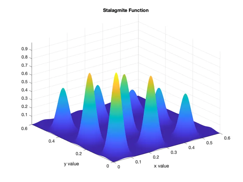
Firstly we will create our own function to calculate the value of objective function at various values of x and y

we use linspace command for creating various x and y values

Now,we create a matrix using the meshgrid function

Now the values in the different matrixs created can be put as an input into the function that we have created,by calling it.By this we can get

the value of the function at various values of x and y

Now since we have got the value of the function at various values.we now need to calculate the maximum value.which can be calculated

using the ga, which is an in-built function

So,for our first study we will use the for loop and iterate it 50 times

We will use the following syntax

[inputs,fopt] = ga(function,number of variables)

here the number of variables are 2 that is x and y

In inputs we will get 1*2 matrix for each iteration, it will basically give the value of x and y and fopt will give the optimum value of the

function at these x and y values

These innuts can he stored and we can use the surf command to create a surface to visualize the function

We can also use the marker command to find the points of local maximum

tic toc command can be used to look at the time taken for evaluation.

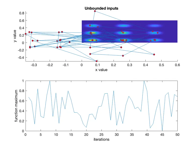
The drawback of this study is that since ga command does not know the bound of these x and y values, so it can take the values greater

than O.6 or less than •

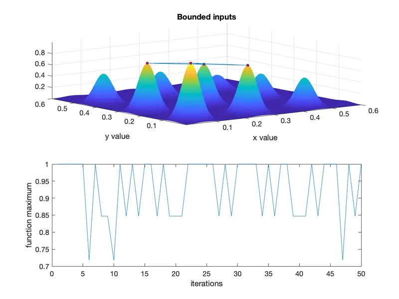
So to overcome this we need to set up a second study which can put restrictions to the value of x and y.Hence we set up upper and lower

bounds for this ga function and the syntax is

[inputs,fopt] = ga(function, number of variables,A,b,Aeq,beq,lb,ub) where

Ib is the lower bound and ub is the upper bound

A -linear inequality constraints

b-linear inequality constraints

Aeq-linear equality constraints

beq-linear equality constraints

since there is no inequality constraints or equality constraints,A,b.Aeg,beg are represented as O

[inputs,fopt] = ga(function, number of variables,O,00.0,lb,ub)

If we execute the loop we will get different local maximas with bounded inputs

But still this is not correct as it is showing local maximas but it is certainlv better than the first study

So to overcome this problem we need to increase the population size as it increases the probability to converge to a global maximum

The syntax that needs to be used is

[inputs,fopt] = ga(function, number of variables,0.0.0.L,lb,ub,I.I.options)

This study can help us to converge to the most accurate solution.

Program :-

% genetic algorithm
% Authored by Nishant Bagal

% Independent variables
x = linspace(0,0.6,150);
y = linspace(0,0.6,150);
% matrix
[xx,yy] = meshgrid(x,y);
% Number of iterations
num_cases = 50;
% Starting the loop
for i = 1:length(xx)
    for j = 1:length(yy)
        input_vector(1) = xx(i,j);
        input_vector(2) = yy(i,j);
        f(i,j) = stalagmite(input_vector);
    end
end
% creates a three dimentional surface
figure(1)
surfc(xx,yy,-f)
shading interp % makes the surface more smoother
xlabel('x value')
ylabel('y value')
title('Stalagmite Function')

% Study 1
tic
for i = 1:num_cases
    [inputs,fopt(i)] = ga(@stalagmite,2);
    xopt(i) = inputs(1);
    yopt(i) = inputs(2);
end
study_1 = toc
figure(2)
subplot(2,1,1)
hold on
surfc(x,y,-f)
title('Unbounded inputs')
xlabel('x value')
ylabel('y value')

shading interp
hold on

plot3(xopt,yopt,-fopt,'Marker','o','markersize',5,'markerfacecolor','r')
subplot(2,1,2)
plot(-fopt)
xlabel('iterations')
ylabel('function maximum')

% case 2nd with upper and lower bounds
tic;
for i = 1:num_cases
    [inputs,fopt(i)] = ga(@stalagmite,2,[],[],[],[],[0;0],[0.6;0.6]);
    xopt(i) = inputs(1);
    yopt(i) = inputs(2);
end
study_2_time = toc
figure(3)
subplot(2,1,1)
surfc(x,y,-f)
shading interp
title('Bounded inputs')
xlabel('x value')
ylabel('y value')

hold on

plot3(xopt,yopt,-fopt,'marker','o','markersize',4,'markerfacecolor','r')
subplot(2,1,2)
plot(-fopt) % plotting -f vs number of iterations
xlabel('iterations')
ylabel('function maximum')

Global_Maxima = -fopt

Function :-

function [f] = stalagmite(input_vector)

a = input_vector(1);
b = input_vector(2);

term1 = (sin((5.1*pi*a)+0.5))^6;
term2 = exp(-4*log(2)*((a-0.0667)^2)/0.64);
term3 = (sin((5.1*pi*b)+0.5))^6;
term4 = exp((-4)*log(2)*((b-0.0667)^2)/0.64);

[f] = -(term1*term2*term3*term4);  %inverts the objective function
end

Results :-