Week 4.1 - Genetic Algorithm

Genetic Algorithm

A genetic algorithm is a search heuristic that is inspired by Charles Darwin’s theory of natural evolution. This algorithm reflects the process of natural selection where the fittest individuals are selected for reproduction in order to produce offspring of the next generation.

This method for solving both constrained and unconstrained optimization problems is based on natural selection, the process that drives biological evolution. The genetic algorithm repeatedly modifies a population of individual solutions.

Natural selection

The process of natural selection starts with the selection of the fittest individuals from a population. They produce offspring which inherit the characteristics of the parents and will be added to the next generation. If parents have better fitness, their offspring will be better than parents and have a better chance at surviving. This process keeps on iterating and in the end, a generation with the fittest individuals will be found.

Five phases are considered in a genetic algorithm.

1. Initial population
2. Fitness function
3. Selection
4. Crossover
5. Mutation

Initial population

The process begins with a set of individuals which is called a Population. Each individual is a solution to the problem you want to solve.

An individual is characterized by a set of parameters (variables) known as Genes. Genes are joined into a string to form a Chromosome (solution).

In a genetic algorithm, the set of genes of an individual is represented using a string, in terms of an alphabet. Usually, binary values are used (string of 1s and 0s). We say that we encode the genes in a chromosome.

fitness function

The fitness function determines how to fit an individual is (the ability of an individual to compete with other individuals). It gives a fitness score to each individual. The probability that an individual will be selected for reproduction is based on its fitness score.

selection

The idea of the selection phase is to select the fittest individuals and let them pass their genes to the next generation.

Two pairs of individuals (parents) are selected based on their fitness scores. Individuals with high fitness have more chances to be selected for reproduction.

Selection rules select the individuals, called parents, that contribute to the population at the next generation.

Crossover

Crossover is the most significant phase in a genetic algorithm. For each pair of parents to be mated, a crossover point is chosen at random from within the genes.

Offspring are created by exchanging the genes of parents among themselves until the crossover point is reached.

The new offspring are added to the population.

Crossover rules combine two parents to form children for the next generation.

mutation

In certain new offspring formed, some of their genes can be subjected to a mutation with a low random probability. This implies that some of the bits in the bit string can be flipped.

Mutation rules apply random changes to individual parents to form children.

how genetic algorithm actually works, which basically tries to mimic human evolution to some extent.

So to formalize a definition of a genetic algorithm, we can say that it is an optimization technique, which tries to find out such values of input so that we get the best output values or results.

The working of a genetic algorithm is also derived from biology, which is shown in the image below.

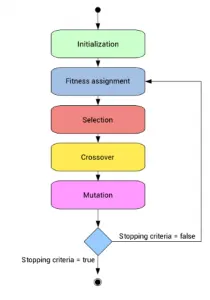
the above line flow diagram for the genetic algorithm

Application

in real world

Genetic algorithm has many applications in the real world. Here I have listed some of the interesting applications, but explaining each one of them will require me an extra article.

Engineering Design

Engineering design has relied heavily on computer modelling and simulation to make the design cycle process fast and economical. A genetic algorithm has been used to optimize and provide a robust solution.

Genetic Algorithm ( GA)

ft=ga(fun,nvars,A,b)

finds a local minimum x to fun, subject to the linear inequalities A*x ≤ b. ga evaluates the matrix product A*x as if x is transposed (A*x').

ft = ga(fun,nvars,A,b,Aeq,beq,lb,ub) defines a set of lower and upper bounds on the design variables, x, so that a solution is found in the range lb ≤ x ≤ ub. (Set Aeq=[] and beq=[] if no linear equalities exist.)

ft=ga(fun,nvars,A,b,Aeq,beq,lb,ub,nonlcon,options)minimizes with the default optimization parameters replaced by values in options. (Set nonlcon=[] if no nonlinear constraints exist.) Create options using optimoptions.

ga=Genetic Algorithm

fun=function to solve the equation

nvars= number of output variables (2)

A= Linear inequality constraints real vector []

b= Linear inequality constraints real vector []

Aeq= Linear inequality constraints real matrix []

beq= Linear inequality constraints real vector []

form Aeq*x = beq

lb= lower Bounce [0;0]

ub= Upper Bounce [1;1]

nonlcon= Nonlinear constraints, specified as a function handle or function name []

options = optimoptions(SolverName,Name,Value) returns options with the named parameters altered with the specified values.

SolverName= population size

Stalagmite

Stalactites, the most familiar structures found hanging from the ceilings of limestone caves, grow by
the precipitation of calcium carbonate from within a thin film of fluid flowing down their surfaces.

Stalactite growth as a free-boundary problem

Equation.

`F_(1x)=(sin(5.1*pi*x +0.5))^6`

`F_(1y)=(sin(5.1*pi*y +0.5))^6`

`F_(2x)=exp((-4*log(2))*((x-0.0667)^2/0.64))`

`F_(2y)=exp((-4*log(2))*((y-0.0667)^2/0.64))`

`f=-(F_(1x)*F_(1y)*F_(2x)*F_(2y))`

MATLAB CODE

Function

function f=stalagmite(input_vector)
x=input_vector(1);
y=input_vector(2);

F1x=(sin(5.1*pi*x +0.5))^6;
F1y=(sin(5.1*pi*y +0.5))^6;
F2x=exp((-4*log(2))*((x-0.0667)^2/0.64));
F2y=exp((-4*log(2))*((y-0.0667)^2/0.64));

f=-(F1x*F1y*F2x*F2y);
end

Main Coad

clear all;
close all;
clc;

% defining our search space
x=linspace(0,0.6,150);
y=linspace(0,0.6,150);

%Iteration 
n=50 % number of iteration

% creating 2D mesh
[xx yy] = meshgrid(x,y);


%evaluating the stalagmite function
for i = 1:length(xx)
    for j= 1:length(yy)
        input_vector(1)=xx(i,j);
        input_vector(2)=yy(i,j);
        f(i,j)= stalagmite(input_vector);
    end
end 
% case 1 unbound condition
tic
for i=1:n
    [input, ft(i)] = ga(@stalagmite,2);
    
    xt(i)=input(1);
    yt(i)=input(2);
end
% time taken for case to analysis
case1=toc

figure(1)
subplot(2,1,1)
hold on
surfc(xx,yy,-f)
shading interp
plot3(xt,yt,-ft,'-o','markersize',3,'markerfacecolor','m')
xlabel('x value')
ylabel('y value')
zlabel('stalagmite function')
title('unbounded stalagmite function')
subplot(2,1,2)
plot(-ft)
xlabel('Iteration')
ylabel('stalagmite function')

%case 2 static behaviour with upper and lower bounce
tic
for i=1:n
    [input, ft(i)] = ga(@stalagmite,2,[],[],[],[],[0;0],[1;1]);
    
    xt(i)=input(1);
    yt(i)=input(2);
end
% time taken for case to analysis
case2=toc;


figure(2)
subplot(2,1,1)
hold on
surfc(xx,yy,-f)
shading interp
plot3(xt,yt,-ft,'-o','markersize',3,'markerfacecolor','m')
xlabel('x value')
ylabel('y value')
zlabel('stalagmite function')
title('Bounded stalagmite function')
subplot(2,1,2)
plot(-ft)
xlabel('Iteration')
ylabel('stalagmite function')

%case 3 increasing GA iteration
options = optimoptions('ga')
options = optimoptions(options,'PopulationSize',350);

tic
for i=1:n
    [input, ft(i)] = ga(@stalagmite,2,[],[],[],[],[0;0],[1;1],[],[],options);
    
    xt(i)=input(1);
    yt(i)=input(2);
end
% time taken for case to analysis
case3=toc;


figure(3)
subplot(2,1,1)
hold on
surfc(xx,yy,-f)
shading interp
plot3(xt,yt,-ft,'-o','markersize',3,'markerfacecolor','m')
xlabel('x value')
ylabel('y value')
zlabel('stalagmite function')
title('Bounded input Modified Population Size')
subplot(2,1,2)
plot(-ft)
xlabel('Iteration')
ylabel('stalagmite function')

Graph output

case1 unbounded condition

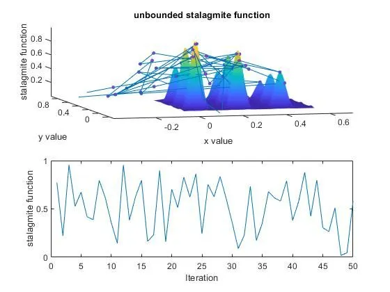
The initial run case1 we can find bounce value to extract global maximum value here we find maximum value false in range 0 to 1

where the time is taken for 50 iterations is= 2.4356 s

Case2 bounded condition with upper and lower condition

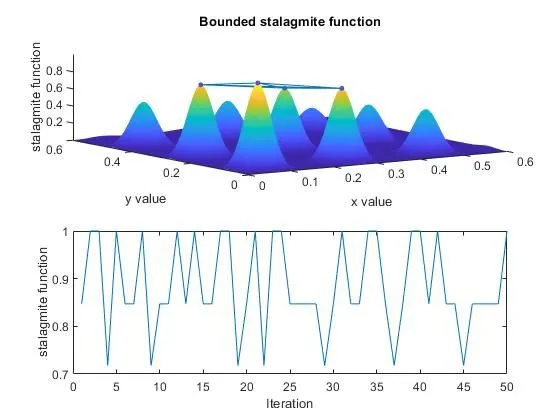
constraining the value of the global maximum 0 to 1 where minimize global maximize value in the range here it is 4 value

time took 3.4725 S

case3 bounded condition with population

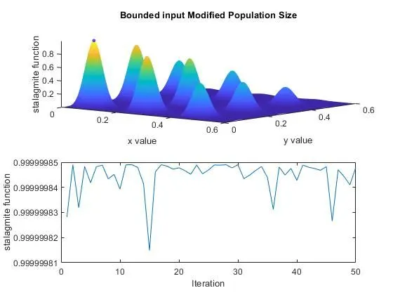
Property solving

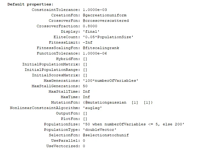
further population size technic Examine the first 350 members of the final population and their corresponding scores. to further minimize the global maximum value higher the value

time took =14.9126

conclusion

where from population technic we can extract the global maximum value x=0.06683,y=0.06683, global maxima stalagmite function=0.9999985

In population technic when we increase the population number value global maximum value decreases and maximum time to solve the value. when we decrease population time taken to solve is lesser and the number of global maximum options is more so we can constrain and play to get value of global maximum

the negative function of function output can find maximum value -f,-ft

References

https://towardsdatascience.com/introduction-to-genetic-algorithms-including-example-code-e396e98d8bf3

https://in.mathworks.com/help/gads/what-is-the-genetic-algorithm.html

https://www.damtp.cam.ac.uk/user/gold/pdfs/stalactite_long.pdf