Week 4.1 - Genetic Algorithm
Concept of Genetic Algorithm:
Optimization:
Optimization is finding the best results under a set of prioritized criteria or constraints.
The parameters included in optimization are:
- Variables: Parameters that will have to be varied during the optimization process are known as variables.
- Constraints: The limits for the output of optimization are known as constraints.
- Objective function: It is a mathematical function or a formula that includes all variables as inputs. The Genetic Algorithm is one of the objective functions.
- Variable bounds: They are the range of input variables that can be varied to provide an optimized result.
Genetic Algorithm:
It is one of the optimization algorithms which is based on the principle of genetics and natural selection.
The process of selection starts with the selection of the fittest individuals from a population.
The best set of solutions is taken into consideration.
There are 5 steps in a genetic algorithm:
- Initial population
- Fitness function
- Selection
- Cross over
- Mutation
- Initial population: The process begins with an initial population. Each individual is a solution to the problem to be solved.
- Fitness function: It determines how close a given solution is to the optimum solution of the desired problem. It determines the fitness of the solution. In a genetic algorithm, each solution is generally represented as a string of binary numbers. Each solution is given a fitness score which is obtained by applying the fitness function to the test.
- Selection: The solution is selected considering the fitness score. Individuals with the highest fitness score are selected.
- Cross over and Mutation: Mutation enables strings to be changed in order to maintain diversity within the population. It enables to produce a superior offspring. The mutation also helps in terminating the population to avoid it entering the local minima. It happens if it doesn't produce a significantly diverse generation since the population is of a fixed size.
The syntax for ga:
x=ga (fun, nvars)
x=ga (fun, nvars, A, b)
x=ga (fun, nvars, A, b, Aeq, beq)
x=ga (fun, nvars, A, b, Aeq, beq, lb, ub)
x=ga (fun, nvars, A, b, Aeq, beq, lb, ub, nonlcon)
x=ga (fun, nvars, A, b, [], [], lb, ub, nonlcon, IntCon)
x=ga (fun, nvars, A, b, [], [], lb, ub, nonlcon, IntCon, Options)
x= ga (_)
[x, fval] = ga (_)
[x, fval, exitflag, output] = ga (_)
[x, fval, exitflag, output, population, scores] = ga (_)
where,
x=optimum solution or variables
A,b=linear inequality constraints
Aeq,beq= linear equality constraints
lb = lower bound
ub = upper bound
nonclon = nonlinear constraints
IntCon = Integer constraints
Stalagmite function:
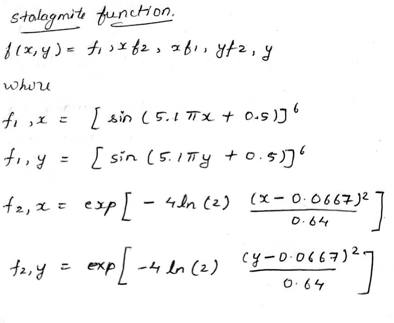
The stalagmite structures are formed from the cave floor which is pointed upwards. The stalagmite function is a mathematical function that represents the shape of a stalagmite. The stalagmite function is defined as:
Code to optimize and find the global minima
%Program on genetic algorithm and stalagmite function

clear all
close all
clc

x=linspace(0,0.6,150);
y=linspace(0,0.6,150);

%Creating a 2-D array
[xx yy]=meshgrid(x,y)

%Evaluating the stalagmite function
for i=1:length(xx)
    for j=1:length(yy)
        input_vector(1)=xx(i,j);
        input_vector(2)=yy(i,j);
        f(i,j)=stalagmite(input_vector);
    end
end

surfc(xx,yy,f)
shading interp
xlabel('x value')
ylabel('y value')
[x,fval]=ga(@stalagmite,2)
title ('Stalagmite main program')
Program for stalagmite function for global minima
%Program of the stalagmite function

function[f]=stalagmite(input_vector)
x=input_vector(1);
y=input_vector(2);
f1=(sin(5.1*pi*x+0.5))^6;
f2=(sin(5.1*pi*y+0.5))^6;
f3=exp(-4*log(1)*(x-0.0667)^2/0.64);
f4=exp(-4*log(2)*(x-0.0667)^2/0.64);
f=(f1*f2*f3*f4)
end
Explanation:
- The 1-Dimensional and 2-Dimensional arrays are created.
- The 2-D array is created using the meshgrid command
- The for loop is used evaluate the stalagmite function
- The stalagmite using the concept of ga as an inbuilt solver is defined separately as a function and called into the main program.
- The results of stalagmite function is stored in the variable f
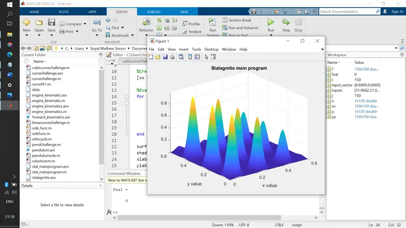
- The surfc command is used to get inputs to the plot and the shading interp command is used to remove gridlines and get a clearer shaded plot.
Output:
Case study
Study of statistical behaviors:
Program to optimise the stalagmite function using ga and get the global maxima along with the plot of Iterations vs F-maximum
%Program on genetic algorithm and stalagmite function

clear all
close all
clc

%Inputs
x=linspace(0,0.6,150);
y=linspace(0,0.6,150);
num_cases=50;

%Creating a 2-D array
[xx yy]=meshgrid(x,y)

%Evaluating the stalagmite function
for i=1:length(xx)
    for j=1:length(yy)
        input_vector(1)=xx(i,j);
        input_vector(2)=yy(i,j);
        f(i,j)=stalagmite(input_vector);
    end
end


%Case study - Number of iterations vs F-maximum
%case 1:

%tic toc commands to find elapsed time
tic
for i=1:num_cases
    [inputs,fopt(i)]=ga(@stalagmite,2);
    xopt(i)=inputs(1);
    yopt(i)=inputs(2);
end
elapsed_time_case_1=toc

%Plotting unbounded graph
figure(1)
subplot(2,1,1)
hold on
surfc(xx,yy,f)
shading interp
xlabel('x value')
ylabel('y value')

%Plotting Iterations vs F-maximum
plot3(xopt,yopt,-fopt,'marker','o','markersize',5,'MarkerFaceColor','r')
subplot(2,1,2)
plot(-fopt)
xlabel('Iterations')
ylabel('F-maximum')
title('Iterations vs F-maximum')


%case 2:
tic
for i=1:num_cases
    [inputs,fopt(i)]=ga(@stalagmite,2,[],[],[],[],[0;0],[1;1]);
    xopt(i)=inputs(1);
    yopt(i)=inputs(2);
end
elapsed_time_case_2=toc

%Plotting unbounded graph
figure(2)
subplot(2,1,1)
hold on
surfc(xx,yy,f)
shading interp
xlabel('x value')
ylabel('y value')

%Plotting Iterations vs F-maximum
plot3(xopt,yopt,-fopt,'marker','o','markersize',5,'MarkerFaceColor','r')
subplot(2,1,2)
plot(-fopt)
xlabel('Iterations')
ylabel('F-maximum')
title('Iterations vs F-maximum')
The code for the stalagmite function to find global maxima:
%Program of the stalagmite function

function[f]=stalagmite(input_vector)
x=input_vector(1);
y=input_vector(2);
f1=(sin(5.1*pi*x+0.5))^6;
f2=(sin(5.1*pi*y+0.5))^6;
f3=exp(-4*log(1)*(x-0.0667)^2/0.64);
f4=exp(-4*log(2)*(x-0.0667)^2/0.64);
f=-(f1*f2*f3*f4)
endExplanation:
- The stalagmite function is defined using the inbuilt ga solver in MATLAB.
- input_vector is taken as the inputs for the stalagmite function
- The results of stalagmite function is stored in the variable f and it is taken as negative (-) because we need to find the global maxima of the function.
Outputs of case study:
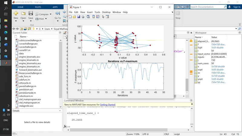
Case 1:
syntax of ga:
ga(@stalagmite,2);
Elapsed time for case 1: 28.2665 sec
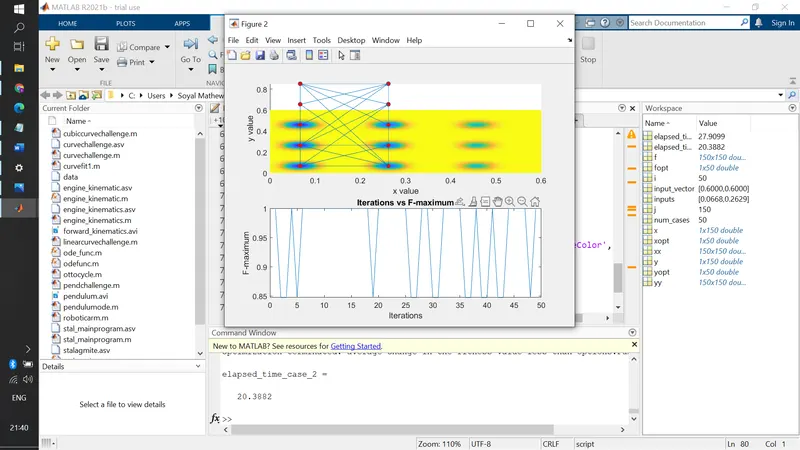
Case 2:
syntax for ga:
ga(@stalagmite,2,[],[],[],[],[0;0],[1;1]);
Elapsed time for case 2: 20.3882 sec
References:
2. https://skill-lync.com/student-projects/Stalagmite-Function-Optimization-77829
3. https://in.mathworks.com/help/gads/genetic-algorithm.html
4. https://skill-lync.com/student-projects/STALAGMITE-FUNCTION-96503
5. https://skill-lync.com/student-projects/Global-Maxima-of-Stalagmite-Function-16698
6. https://www.iitg.ac.in/rkbc/CE602/CE602/Genetic%20Algorithms.pdf
7. https://in.mathworks.com/help/gads/ga.html