Week 4.1 - Genetic Algorithm

MATLAB PROGRAM FOR GA(GENETICN ALGORITHM -

* The search space of the stalagmite function is defined using the "linspace"

* 2-dimensional array is created using 'meshgrid'

* Then to plot the stalgmite function for loop is used & separate function is coded using the following eqns ;

f(x,y) = f1xf2xf1yf2y

f1,x = [sin(6.1*pi*x+0.5)]^6 , f1,y = 'sin(5.1*pi*y+0.5)]^6

f2,x = exp[-4 ln(2) ((x-0.0667)^2/0.64)

f2,y = exp[-4 ln(2) ((y-0.0667)^2/0.64)

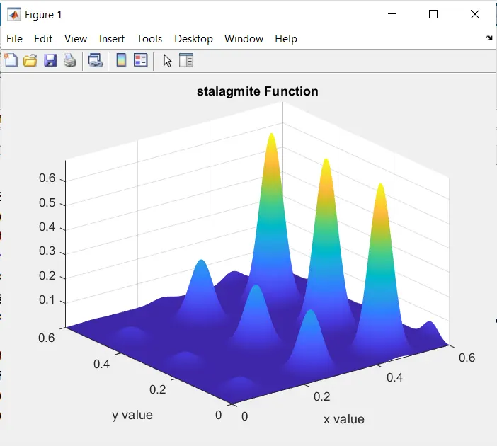
* Then the stalagmite function is plotted using the 'SurfC' command & the output graph is obtained.

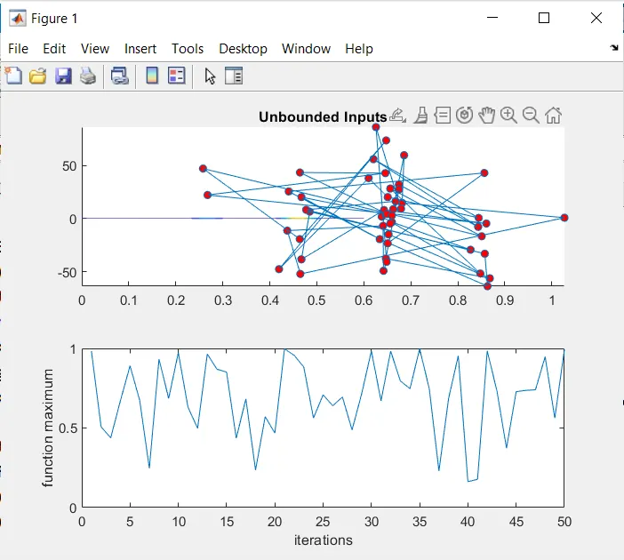
* Then the 1st study with unbounded inputs are given using the GENETIC ALGORITHM which is inbuilt matlab function.

* The total time of evaluation is calculated using tic toc command.

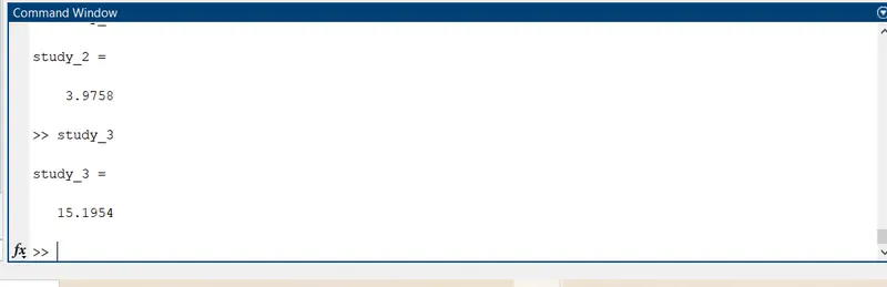
* Then thesame procedure is repeated for the next two studies by giving the lower & Upper bounds foer study2 & by increasing the number of iterations & giving the population size for study3

SYNTAX FOR GENETIC ALGORITHM-

* x = ga(func,nvars)-

finds a local unconstrained minimum,x,to the objective functiion,func.nvars is the dimension (number of design variables0 OF FUNC.

* x = ga(func,nvars,A,b,Aeq,beq,lb,ub)-

defnes a set of lower & upper bounds on the design variables,x,so that a solution is found in the range lb <x<ub.(set Aeq=[] & beq=[] if no linear equalities exist.)

* x = ga(func,nvars,A,b,[],[],lb,ub,nonlcon,lntcon,options)-

Requires that the variables listed in lntcon take integer values.

Where,

x = local minimum

func - objective function

nvars - number of variables

A - linear inequality constraints

B - linear inequality constraints

Aeq - linear equality constraints

Beq - linear equality constraints

lb - lower bounds

ub - upper bounds

nonlcon - non-linear constraints

lntcon - integer values

options - optimization options

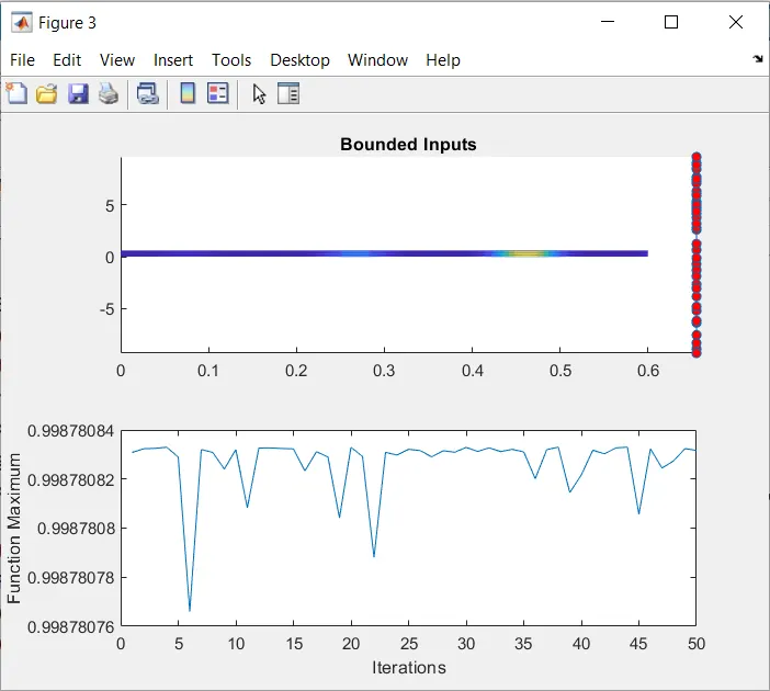
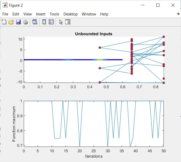
The three cases considerd fopr Fmax vs no of iterations,

1. Unbounded inputs-No input restrictions.

2. Bounded inputs- inputs are restricted with Upper & Lower bounds.

3. Bounded inuputs with options - Increasing no of iterations by giving populations size.

close all
clear all
clc
% defining our search space
x = linspace(0,0.6,150);
y = linspace(0,0.6,150);

% creating a 2-d array
[xx yy] = meshgrid(x,y);
num_cases =  50;

% evaluating the stalagmite function
for i = 1:length(xx)
    for j = 1:length(yy)
      input_vector(1) = xx(i,j);
      input_vector(2) = yy(i,j);
      F(i,j) = stalagmite(input_vector);
    end
end
surfc(xx,yy,-F)
shading interp
xlabel('x value')
ylabel('y value')
title('stalagmite Function')

% study 1
tic
for i = 1:num_cases
    [inputs,Fopt(i)] = ga(@stalagmite,2);
    xopt(i) = inputs(1);
    yopt(i) = inputs(2);
end

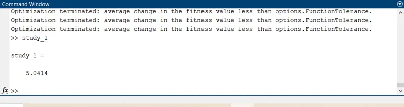
study_1 = toc;
figure(1)
subplot(2,1,1)
hold on
surfc(x,y,-F)
shading interp
plot3(xopt,yopt,-Fopt,'Marker','o','MarkerSize',5,'MarkerFaceColor','r')
title('Unbounded Inputs')
subplot(2,1,2)
plot(-Fopt)
xlabel('iterations')
ylabel('function maximum')


% study_2
tic
for i = 1:num_cases
    [inputs,Fopt(i)] = ga(@stalagmite,2,[],[],[],[],[0:0],[1:1]);
    xopt(i) = inputs(1);
    yopt(i) = inputs(2);
end
study_2 = toc;
figure(2)
subplot(2,1,1)
hold on
surfc(x,y,-F)
shading interp
plot3(xopt,yopt,-Fopt,'marker','o','markersize',5,'MarkerFaceColor','r')
title('Unbounded Inputs')
subplot(2,1,2)
plot(-Fopt)
xlabel('Iterations')
ylabel('Function maximum')


% study3
options = optimoptions(@ga);
options = optimoptions(options,'PopulationSize',400);

tic
for i = 1:num_cases
    [inputs,Fopt(i)] = ga(@stalagmite,2,[],[],[],[],[0:0],[1:1],[],[],options);
    xopt(i) = inputs(1);
    yopt(i) = inputs(2);
end

study_3 = toc;
figure(3)
subplot(2,1,1)
hold on 
surfc(x,y,-F)
shading interp
plot3(xopt,yopt,-Fopt,'marker','o','MarkerSize',5,'MarkerFaceColor','r')
title('Bounded Inputs')
subplot(2,1,2)
plot(-Fopt)
xlabel('Iterations')
ylabel('Function Maximum')

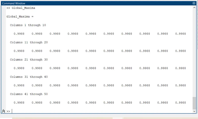
Global_Maxima = -Fopt;

function [F] = stalagmite(input_vector)
a = input_vector(1);
b = input_vector(2);

f1 = (sin((5.1*pi*a)+0.5))^6;
f2 = (sin((5.1*pi*b)+0.5))^6;
f3 = exp((-4*log(2)*((a-0.667)^2))/(0.64));
f4 = exp((-4*log(2)*((a-0.667)^2))/(0.64));

F = -(f1*f2*f3*f4);
end