Week 4.1 - Genetic Algorithm

THEORY:-
What is a Genetic Algorithm:-
A genetic algorithm (GA) is a method for solving both constrained and unconstrained
optimization problems based on a natural selection process that mimics biological
evolution. The algorithm repeatedly modifies a population of individual solutions. At
each step, the genetic algorithm randomly selects individuals from the current
population and uses them as parents to produce the children for the next generation.
Over successive generations, the population "evolves" toward an optimal solution.

You can apply the genetic algorithm to solve problems that are not well suited for
standard optimization algorithms, including problems in which the objective function is
discontinuous, nondifferentiable, stochastic, or highly nonlinear.
The genetic algorithm differs from a classical, derivative-based, optimization algorithm in
two main ways, as summarized below.
Classical Algorithm:-
● Generates a single point at each iteration.
● The sequence of points approaches an optimal solution.
● Selects the next point in the sequence by a deterministic computation.
Genetic Algorithm:-
● Generates a population of points at each iteration.
● The best point in the population approaches an optimal solution.
● Selects the next population by computation which uses random number
generators.

Stopping Criteria of Genetic Algorithm:-
Proof of convergence of an algorithm to an optimal solution is very important as it
assures the optimal solution in infinite iterations. When an algorithm does not assure or
guarantee the optimal solution even after running for infinite iterations, its utility is in
doubt. Once the convergence of an algorithm is assured, the focus turns into the
exploration of the stopping time or stopping criterion of the algorithm. Today, the biggest
challenge in the implementation of GAs is to decide when to stop the algorithm keeping
in mind that there is no a-prior information regarding the objective function. Attempts
have been made to provide stopping criteria of a GA based on the time the algorithm is
being executed and obtained objective function values or their distribution [11, 8, 12].
Time-based stopping criteria are mainly of two kinds. The popular one is to decide
upfront the number of iterations to be executed. Another is based on the execution time
of the algorithm. An algorithm is run for a predetermined period and gets the result.
Though these criteria are very simple to implement but determining the time is again a
challenge.
The theoretical study brings out a number of limitations in defining a stopping criterion.
Some desirable properties of a ”good” stopping criterion are given below.
• Easy to implement.
• Able to provide stopping time automatically for any fitness function.
• Should lead to ’good’ / ’satisfactory’ results.

• Total number of strings searched should not exceed 2L

Where GA is used?

Genetic Algorithms are primarily used in optimization problems of various kinds, but
they are frequently used in other application areas as well. The areas in which Genetic
Algorithms are frequently used are listed below.
Optimization - Genetic Algorithms are most commonly used in optimization problems
wherein we have to maximize or minimize a given objective function value under a
given set of constraints.
• Economics - GAs are also used to characterize various economic models like the
cobweb model, game theory equilibrium resolution, asset pricing, etc.
• Neural Networks - GAs are also used to train neural networks, particularly recurrent
neural networks.
• Image Processing - GAs are used for various digital image processing (DIP) tasks as
well as dense pixel matching.
The above are some of the areas where the Genetic Algorithm is extensively used for
optimization.

Syntax of Genetic Algorithm:-
● x = ga(fun,nvars) finds a local unconstrained minimum, x, to the objective
function, fun. nvars is the dimension (number of design variables) of fun.
● x = ga(fun,nvars,A,b,Aeq,beq) finds a local minimum x to fun, subject to the
linear equalities Aeq*x = beq and A*x ≤ b. (Set A=[] and b=[] if no linear
inequalities exist.) ga evaluates the matrix product Aeq*x as if x is transposed
(Aeq*x')
● x = ga(fun,nvars,A,b,Aeq,beq,lb,ub) defines a set of lower and upper
bounds on the design variables, x, so that a solution is found in the range lb ≤ x
≤ ub. (Set Aeq=[] and beq=[] if no linear equalities exist.
● x = ga(fun,nvars,A,b,Aeq,beq,lb,ub,nonlcon) subjects the minimization to
the constraints defined in nonlcon. The function nonlcon accepts x and returns
vectors C and Ceq, representing the nonlinear inequalities and equalities
respectively. ga minimizes the fun such that C(x) ≤ 0 and Ceq(x) = 0. (Set
lb=[] and ub=[] if no bounds exist.)

● x = ga(fun,nvars,A,b,Aeq,beq,lb,ub,nonlcon,options) minimizes with the
default optimization parameters replaced by values in options. (Set nonlcon=[]
if no nonlinear constraints exist.) Create options using optimization.
● x = ga(fun,nvars,A,b,Aeq,beq,lb,ub,nonlcon,intcon) or x =
ga(fun,nvars,A,b,Aeq,beq,lb,ub,nonlcon,intcon,options) requires that the
variables listed in intcon take integer values
● x = ga(problem) find the minimum for, a structure described in the problem.
● [x,fval] = ga(___), for any previous input arguments, also returns fval, the
value of the fitness function at x
● [x,fval,exitflag,output] = ga(___) also returns exitflag, an integer
identifying the reason the algorithm terminated, and output, a structure that
contains output from each generation and other information about the
performance of the algorithm.
● [x,fval,exitflag,output,population,scores] = ga(___) also returns a
matrix population, whose rows are the final population, and a vector scores, the
scores of the final population.

MATLAB PROGRAMMING:-
Function Code:-

● here the stalagmite function consists of 4 different functions which have been
calculated separately along with their product as f which we can see in the above
code.
● This function helps us to get the values of the global minima and global maxima
of a stalagmite function when called upon in the main program as a function
code.
● However, with this function, it gives us the global maxima whereas in other
cases, when we want to achieve the global minima, there is a slight difference
where we remove the -ve sign on the output variable notation.

% function of stalagmite 

function  f=stalagmite(input_vector)
x=input_vector(1);
y=input_vector(2);
f1 = (sin(5.1*pi*x+0.5))^6;
f2= (sin(5.1*pi*y+0.5))^6;

f3= exp(-4*log(2)*((x-0.0667)^2)/(0.64));
f4= exp(-4*log(2)*((y-0.0667)^2)/(0.64));

f= -(f1*f2*f3*f4);
end
  

Main Code:-

● The main program consists of three different studies with these we are able to
get the values of global minima and global maxima.
● For the first case, statistical behavior is checked where no values of bounds are
provided.
● For the second case, statistical behavior is checked where values of upper and
lower bounds are provided.
● And for the third case, the genetic algorithm interactions are increasing to get the
values of global minima and global maxima.
● To reduce the run time of the given program it's best to run individual cases at a
time with this the output we get is easy to study.
● The main code is given below.

clear all
close all
clc

% Defining search space
x = linspace(0,0.6,150);
y = linspace(0,0.6,150);
num_cases = 50;


% creating 2D array using meshgrid
[xx,yy] = meshgrid(x,y);

% evaluating the stalagmite function
for i=1:length(xx)
    for j=1:length(yy)
        input_vector(1)=xx(i,j);
        input_vector(2)=yy(i,j);
        f(i,j)=stalagmite(input_vector);
    end
end
tic

% study 1 - satistical behavior
for i=1:num_cases
    [inputs,fopt1(i)] = ga(@stalagmite,2);
    xopt1(i) = inputs(1);
    yopt1(i) = inputs(2);
end

study1_time = toc;

figure(1)
subplot(2,1,1)
hold on
surfc(x,y,f)
shading interp
plot3(xopt1,yopt1,fopt1,'marker','o','markersize',5,'markerfacecolor','r')
title('Unbounded inputs')
subplot(2,1,2)
plot(fopt1)
xlabel('Iterations')
ylabel('Function minimum')

tic

% study 2 - satistical behavior - with upper and lower bounds

for i = 1:num_cases
    [inputs,fopt(i)] = ga(@stalagmite,2,[],[],[],[],[0;0],[0.6;0.6]);
    xopt(i) = inputs(1);
    yopt(i) = inputs(2);
end

study2_time = toc;

figure(2)
subplot(2,1,1)
hold on
surfc(x,y,f)
shading interp
plot3(xopt,yopt,fopt,'marker','o','markersize',5,'markerfacecolor','r')
title('Unbounded inputs')
subplot(2,1,2)
plot(fopt)
xlabel('Iterations')
ylabel('Function minimum')

% study 3 - increasing GA interations

options = optimoptions('ga','PopulationSize',150);

tic

for i = 1:num_cases
    [inputs,fopt(i)] = ga(@stalagmite,2,[],[],[],[],[0;0],[0.6;0.6],[],[],options);
    xopt(i) = inputs(1);
    yopt(i) = inputs(2);
end

study3_time = toc;    

figure(3)
subplot(2,1,1)
hold on
surfc(x,y,f)
shading interp
plot3(xopt,yopt,fopt,'marker','o','markersize',5,'markerfacecolor','r')
title('Unbounded inputs')
subplot(2,1,2)
plot(fopt)
xlabel('Iterations')
ylabel('Function minimum')

After running the program we got three outputs for our main programming, the output
result is explained below.

RESULTS/OUTPUT:-
1. FOR THE FIRST CASE:-
● For the first case we are going to analysis of genetic algorithm for statistical
behaviour.
● Here for loop is used in this for loop we used ga command on stalagmite function
to reduce the variation of functions.
● We used tic and tac command to provide time taken on a program to run.
● subplot command is used to display output in one single window.
● Here by providing negative value (-ve) we can get global maxima as we mention
early in the theoretical part.

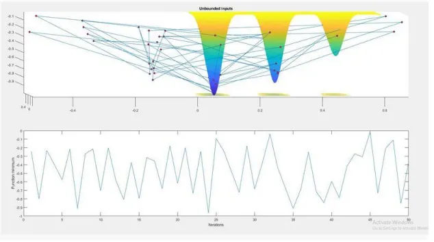
● here as we can see from the above result, the iterations are generating a lots of
values causes a variations.
● To get the less iterations values and less variations we need to provide some
values at their bounds.
● It is impossible to get the exact global maxima due to lots of values.
2. FOR THE SECOND CASE:-
● For the second case we are going to analysis of genetic algorithm for statistical
behaviour with upper bound and lower bound.
● With the help of upper and lower bounds we get the better result as compared to
the first case.
● All the process is same as first case except the UB and LB values are provided
as [inputs,fopt2(i)] = ga(@stalagmite,2,[],[],[],[],[0;0],[0.6;0.6]);

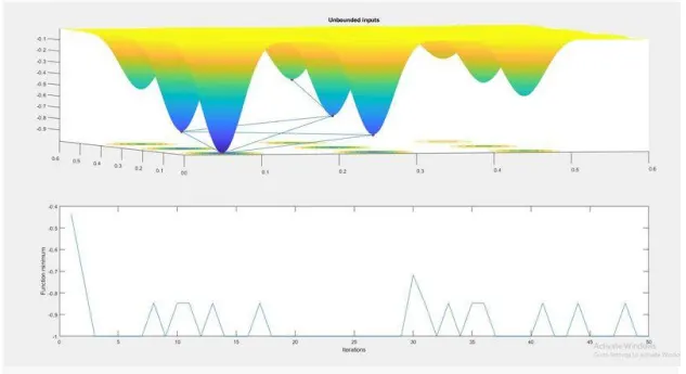
● Here as we can see from the result the iterations are generating less values as
compared to the first case
● Becouse of this variations are also less.
● Only five iterations values are generating here because of this it is easy to find
local and global maxima.
● just because we provided upper and lower bounds we are able to get this much
of less values.
3. FOR THE THIRD CASE:-
● For the third case we are going to analysis of genetic algorithm for increasing
genetic iterations.
● All the process is same as second case except the GA iterations are increasing.
● the GA syntax we used is [inputs,fopt3(i)] =
ga(@stalagmite,2,[],[],[],[],[0;0],[0.6;0.6],[],[],options);
● Here option is helps us to increase the population to increase the size.

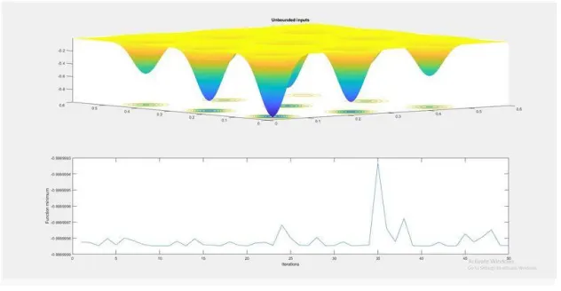
● Here as we can see from the result the iterations are generating only one values
compared to the second case.
● here we get the only one global point for global maxima .
● Also the variation is less than second case.
● This is how genetic algorithm is performed on different values to get the exact
one global maxima.
CONCLUSION:-
Here with the help of MATLAB we understand the concept of the genetic algorithm by
referring to various sources before you attend this challenge and successfully get the
value of global maxima.