Week 4.1 - Genetic Algorithm
INTRODUCTION TO OPTIMIZATION: optimization is the process of finding "best values" of some objective function given a defined domain/input, including a variety of objective functions or different types of domain.
the above image gives the general layout for the optimization process. For a given set of inputs, we get outputs through a defined process. The process of selecting the input that gives the best output value is known as optimization. Mathematically speaking an optimization problem consists of maximizing or minimizing a real function by systematically choosing input values from within an allowed set and computing the value of the function.
A stalagmite function generally refers to the function with which we are generating values over a stalagmite kind of surface for finding out the local and global maxima and minima of that particularly given function.
A maximum or minimum is said to be local if it is the largest or smallest value of the function, respectively, within a given range.
However, a maximum or minimum is said to be global if it is the largest or smallest value of the function, respectively, on the entire domain of a function.
From the above image, the global maxima and local maxima are clearly understood where global maxima are obtained over a domain but local maxima are obtained over a given range or subset of the domain.
Optimization is carried out to find the maxima of a given function and is done by choosing input values systematically from a domain and computing the results of the function.
To perform such a process using Matlab we use the Genetic Algorithm method, which is an inbuilt tool to find the global maxima for the defined stalagmite function.
GENETIC ALGORITHM: A genetic algorithm (GA) is a metaheuristic inspired by the process of natural selection that belongs to the larger class of evolutionary algorithms(EA). Genetic algorithms are commonly used to generate high-quality solutions to optimization and search problems by relying on biologically inspired operators such as mutation, crossover, and selection.
A genetic algorithm (GA) is a method for solving both constrained and unconstrained optimization problems based on a natural selection process that mimics biological evolution. Similar to the evolution process, the algorithm repeatedly modifies a population of individual solutions. At each step, the genetic algorithm randomly selects individuals from the current population and uses them as parents to produce the children for the next generation. Over successive generations, the population "evolves" toward an optimal solution.
we apply the genetic algorithm to solve problems that are not well suited for standard optimization algorithms, including problems in which the objective function is discontinuous, nondifferentiable, stochastic, or highly nonlinear.
In GA we will have a large population with possible solutions for a set of a given problem, these solutions undergo a crossover process producing a variety of solutions. during the crossover process, the mutations occur and these mutations are carried out for over generations. As each of these individuals will be assigned the fitness value, the survival of the fittest by Charles Darwin is employed here and the individual with the highest fitness value shall survive.
GA attempts to find global minima or maxima of a function f(x). it is usually described as the minimization process because the maximization of a real-valued problem g(x) is equivalent to the minimization of the function f(x) = (-1)*g(x).
This way the process is carried out till the evolvement of the individual is better or till we reach the stop criterion.
A typical genetic algorithm requires:
- a genetic representation of the solution domain,
2. a fitness function to evaluate the solution domain. As the genetic representation and fitness function is defined, GA is carried out in the following stages :
- Initialization
- Fitness function
- Selection
- Cross over
- Mutation
Initialization: GA begins with this process with the size of the population(individual). depending on the nature of the problem, there could be several possible solutions. the initial population is generated randomly, allowing the entire range of possible solutions.
Fitness Function: A particular type of objective function which is used to characterize the performance of a function on how close the obtained solution is to achieving the set of given conditions or set aims. Fitness functions are used in GA to guide simulations towards optimal design solutions. The fitness function is defined over the genetic representation and measures the quality of the represented solution, also it is problem-dependent.
Selection: During each successive generation, a part of the existing population is selected to breed a new generation. Individual solutions are selected through a fitness-based process(Roulette wheel selection), where fitter solutions are typically more likely to be selected which are measured by the fitness function.
Cross over: In GA a cross over is a genetic operator that is used to combine the genetic information obtained from the two individual parents during the generation of a new offspring. One way is to stochastically generate new solutions from an existing population, it is the analogous procedure to the crossover that happens during the reproduction process.
Mutation: it is a genetic operator employed to maintain genetic diversity over generations. The purpose of mutation in GAs is to introduce diversity into the sampled population. Mutation operators are used in an attempt to avoid local minima by preventing the population of chromosomes from becoming too similar to each other, thus slowing or even stopping convergence to the global optimum. This reasoning also leads most GA systems to avoid only taking the fittest of the population in generating the next generation, but rather selecting a random set with a weighting toward those that are fitter.
SYNTAX FOR GENETIC ALGORITHM USED IN MATLAB
x = ga(problem) finds the minimum for problem, where problem is a structure
[x,fval]= ga(problem) for any previous input arguments, also returns fval, the value of the fitness function at x.
x = ga(fun,nvars,A,b,Aeq,beq,lb,ub,options) minimizes with the default optimization parameters replaced by values in options. Create options using optimoptions.
CODE TO OPTIMIZE STALAGMITE FUNCTION
STEP 1: Using basic commands to clear previous simulations
clear all %to clear workspace
close all %to close plots
clc %clear command window
STEP 2: to initialize the x & y values by taking 150 in the intrval between 0-0.6 by considering the number cases as 150
% to define search space
x= linspace(0,0.6,150); %1D array in x direction
y= linspace(0,0.6,150); %1D array in y direction
num_cases=50;
%to create a 2D mesh
[xx yy]= meshgrid(x,y);
As we plot a 3D image we consider the 2D array, initializing it through 'meshgrid' command and storing it in input_vector and is used as an argument in defining the stalagmite function.
STEP 3: Calling of stalagmite function
As we shall define the stalagmite function seperately we write the outputs using - ve sign as GA gives only the minimum value. but the negation gives the maximum values(detailed explanation given above).
% Evaluating the stalagmite function
%nested loop for inputs
for i= 1:length(xx)
for j= 1:length(yy)
input_vector(1)=xx(i,j);
input_vector(2)=yy(i,j);
f(i,j)= stalagmite_func(input_vector);
end
end
%% CASE 1 : UNBOUNDED(statistical behaviour)
tic
for i=1:num_cases
[input, fopt(i)]=ga(@stalagmite_func,2);
xopt(i)=input(1);
yopt(i)=input(2);
end
study_1_time=toc;
figure(1)
subplot(2,1,1)
hold on
surfc(x,y,-f)
shading interp
plot3(xopt,yopt,-fopt,'marker','o','markersize',5,'markerfacecolor','r')
title('Unbounded inputs(CASE 1)')
subplot(2,1,2)
plot(-fopt)
xlabel('No of Iterations')
ylabel('Function maximum')
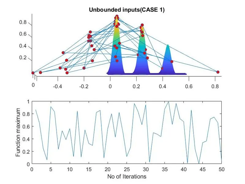
in case study 1 we make use of the ga function which is initialized through the generation of the random population to calculate the maxima of the function. the output is stored in 'fopt'. the results are stored in xopt and yopt, to plot the surface the surfc command is used for obtaining the 3D plot. plot3 is used to plot xopt, yopt and -fopt to get the optimum maximas which are indicated by 'marker'. the tic and toc commands are used to record the time that the ga has used to find the optimal values. case 1 was carried out for the time period of 2.4718s also from the below image it is observed that the x and y values fall out from the surface of the stalagmite function and fail to obtain global maxima. to overcome this drawback we move on to the next case where we define the upper and lower bounds.
STEP 4: to define upper and lower bounds
even though we define the upper and lower bound the GA is still initialized through random population itself.
%% CASE 2: statistical behavior with upper and lower bounds
tic
for i=1:num_cases
[input, fopt(i)]=ga(@stalagmite_func,2,[],[],[],[],[0;0],[0.5;0.5]);
xopt(i)=input(1);
yopt(i)=input(2);
end
study_2_time= toc
figure(2)
subplot(2,1,1)
hold on
surfc(x,y,-f)
shading interp
plot3(xopt,yopt,-fopt,'marker','o','markersize',5,'markerfacecolor','r')
title('Bounded input(CASE 2)')
subplot(2,1,2)
plot(-fopt)
xlabel('No of Iterations')
ylabel('Function maximum')
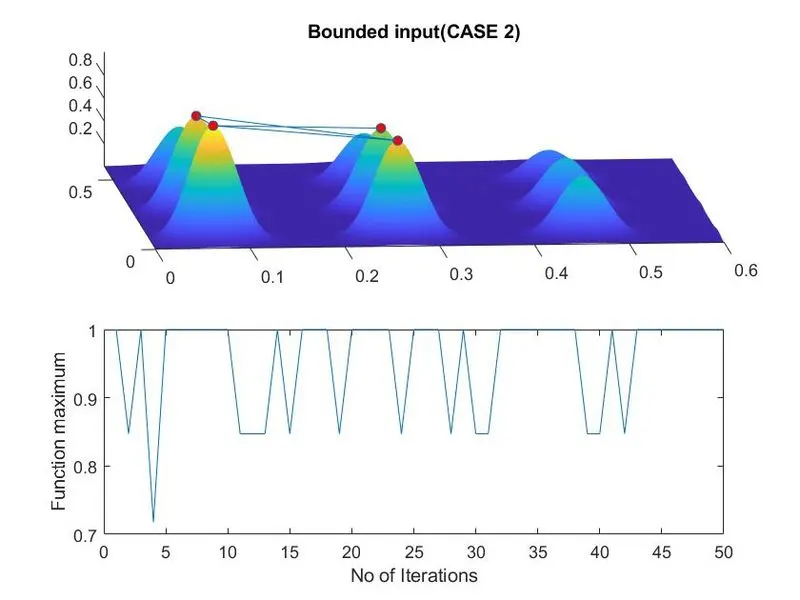
The GA simulation is carried out in a similar way as in case 1 but with the bounds and the time required for ga to carry out is more than the unbound case which is 3.2532 seconds. but it can be seen from the above image that it is still not possible to find global maxima even after defining the bounds though the values are in the optimal bound.
STEP 5: to carry out the GA with population size
at the initial stages we had the population size of about 50 but we icrease it to 170 through 'optimoptions'.
%% CASE 3: increasing GA iterations
options= optimoptions('ga')
options= optimoptions(options,'PopulationSize',170);
tic
for i=1:num_cases
[input, fopt(i)]=ga(@stalagmite_func,2,[],[],[],[],[0;0],[0.5;0.5],[],[],options);
xopt(i)=input(1);
yopt(i)=input(2);
end
study_3_time=toc
figure(3)
subplot(2,1,1)
hold on
surfc(x,y,-f)
shading interp
plot3(xopt,yopt,-fopt,'marker','o','markersize',5,'markerfacecolor','r')
title('Bounded input with population size (CASE 3)')
subplot(2,1,2)
plot(-fopt)
xlabel('No of Iterations')
ylabel('Function maximum')
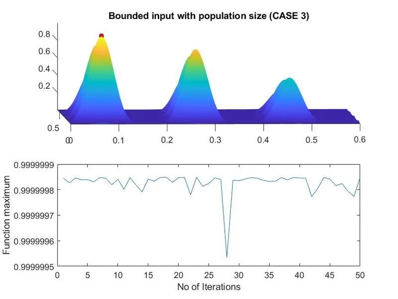
when the study was carried out the ga took a total of 7.4115 seconds to carry out the optimization process. which is more when compared to the other two cases. to get a more accurate result we increase the size of the population.
STEP 6: Increasing the population size
%% CASE 4:
options= optimoptions('ga')
options= optimoptions(options,'PopulationSize',400);
tic
for i=1:num_cases
[input, fopt(i)]=ga(@stalagmite_func,2,[],[],[],[],[0;0],[0.5;0.5],[],[],options);
xopt(i)=input(1);
yopt(i)=input(2);
end
study_4_time=toc
figure(4)
subplot(2,1,1)
hold on
surfc(x,y,-f)
shading interp
plot3(xopt,yopt,-fopt,'marker','o','markersize',5,'markerfacecolor','r')
title('Bounded Input with increased population size(CASE 4)')
subplot(2,1,2)
plot(-fopt)
xlabel('No of Iterations')
ylabel('Function maximum')
display(input) %max x & y values of a function
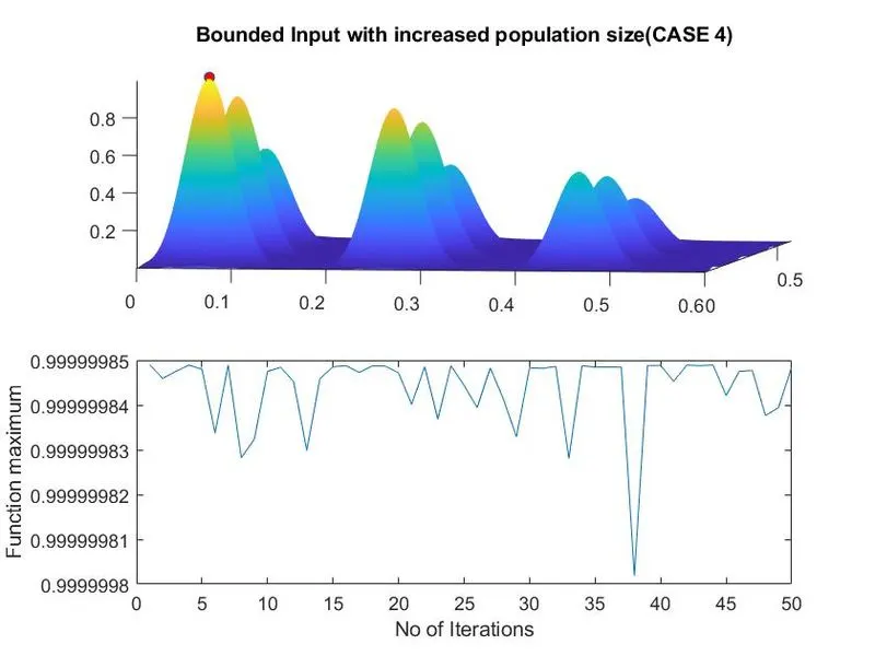
when this process was carried out for the increased population of 400, the ga took a total time of 14.8643 seconds. it is evident that as we increase the population, ga takes a longer time to give the optimal values.
the x and y maximum values are 0.0668 0.0668 respectively.
STEP 7: Stalagmite function
function[f]= stalagmite_func(input_vector) %define stalagmite function
%x= input_vector(1); %input for x
%y= input_vector(2); %input for y
f1x= ((sin((5.1*pi).*input_vector(1)+0.5)).^6); % 1st formula
f1y= ((sin((5.1*pi).*input_vector(2)+0.5)).^6); %2nd formula
f2x= exp(-4*log(2).*(((input_vector(1)-0.0667)^2)/0.64)); %3rd formula
f2y= exp(-4*log(2).*(((input_vector(2)-0.0667)^2)/0.64)); %4th formula
%Stalagmite function is product of all the four formula
f1= (f1x*f1y*f2x*f2y);
f=-f1;
end
code
clear all %to clear workspace
close all %to close plots
clc %clear command window
% to define search space
x= linspace(0,0.6,150); %1D array
y= linspace(0,0.6,150);
num_cases=50;
%to create a 2D mesh
[xx yy]= meshgrid(x,y);
% Evaluating the stalagmite function
%nested loop for inputs
for i= 1:length(xx)
for j= 1:length(yy)
input_vector(1)=xx(i,j);
input_vector(2)=yy(i,j);
f(i,j)= stalagmite_func(input_vector);
end
end
%% CASE 1 : UNBOUNDED(statistical behaviour)
tic
for i=1:num_cases
[input, fopt(i)]=ga(@stalagmite_func,2);
xopt(i)=input(1);
yopt(i)=input(2);
end
study_1_time=toc
figure(1)
subplot(2,1,1)
hold on
surfc(x,y,-f)
shading interp
plot3(xopt,yopt,-fopt,'marker','o','markersize',5,'markerfacecolor','r')
title('Unbounded inputs(CASE 1)')
subplot(2,1,2)
plot(-fopt)
xlabel('No of Iterations')
ylabel('Function maximum')
%% CASE 2 : statistical behaviour with upper and lower bounds
tic
for i=1:num_cases
[input, fopt(i)]=ga(@stalagmite_func,2,[],[],[],[],[0;0],[0.5;0.5]);
xopt(i)=input(1);
yopt(i)=input(2);
end
study_2_time= toc
figure(2)
subplot(2,1,1)
hold on
surfc(x,y,-f)
shading interp
plot3(xopt,yopt,-fopt,'marker','o','markersize',5,'markerfacecolor','r')
title('Bounded input(CASE 2)')
subplot(2,1,2)
plot(-fopt)
xlabel('No of Iterations')
ylabel('Function maximum')
%% CASE 3: increasing GA iterations
options= optimoptions('ga')
options= optimoptions(options,'PopulationSize',170);
tic
for i=1:num_cases
[input, fopt(i)]=ga(@stalagmite_func,2,[],[],[],[],[0;0],[0.5;0.5],[],[],options);
xopt(i)=input(1);
yopt(i)=input(2);
end
study_3_time=toc
figure(3)
subplot(2,1,1)
hold on
surfc(x,y,-f)
shading interp
plot3(xopt,yopt,-fopt,'marker','o','markersize',5,'markerfacecolor','r')
title('Bounded input with population size (CASE 3)')
subplot(2,1,2)
plot(-fopt)
xlabel('No of Iterations')
ylabel('Function maximum')
%% CASE 4:
options= optimoptions('ga')
options= optimoptions(options,'PopulationSize',400);
tic
for i=1:num_cases
[input, fopt(i)]=ga(@stalagmite_func,2,[],[],[],[],[0;0],[0.5;0.5],[],[],options);
xopt(i)=input(1);
yopt(i)=input(2);
end
study_4_time=toc
figure(4)
subplot(2,1,1)
hold on
surfc(x,y,-f)
shading interp
plot3(xopt,yopt,-fopt,'marker','o','markersize',5,'markerfacecolor','r')
title('Bounded Input with increased population size(CASE 4)')
subplot(2,1,2)
plot(-fopt)
xlabel('No of Iterations')
ylabel('Function maximum')
display(input) %max x & y values of a function
STALAGMITE FUNCTION:
function[f]= stalagmite_func(input_vector) %define stalagmite function
%x= input_vector(1); %input for x
%y= input_vector(2); %input for y
f1x= ((sin((5.1*pi).*input_vector(1)+0.5)).^6); % 1st formula
f1y= ((sin((5.1*pi).*input_vector(2)+0.5)).^6); %2nd formula
f2x= exp(-4*log(2).*(((input_vector(1)-0.0667)^2)/0.64)); %3rd formula
f2y= exp(-4*log(2).*(((input_vector(2)-0.0667)^2)/0.64)); %4th formula
%Stalagmite function is product of all the four formula
f1= (f1x*f1y*f2x*f2y);
f=-f1;
end
REFERENCES
[1]https://skill-lync.com/knowledgebase/genetic-algorithm-explained(skill_lync)
[2] https://en.wikipedia.org/wiki/Genetic_algorithm (Wikipedia)
[3] https://de.mathworks.com/discovery/genetic-algorithm.html
clear all                        %to clear workspace
close all                        %to close plots
clc                              %clear command window

% to define search space
x= linspace(0,0.6,150);   %1D array
y= linspace(0,0.6,150);
num_cases=50;

%to create a 2D mesh
[xx yy]= meshgrid(x,y);

% Evaluating the stalagmite function
%nested loop for inputs
for i= 1:length(xx)
    for j= 1:length(yy)
        input_vector(1)=xx(i,j);
        input_vector(2)=yy(i,j);
        f(i,j)= stalagmite_func(input_vector);
    end
end
%% CASE 1 : UNBOUNDED(statistical behaviour)

tic
for i=1:num_cases
    [input, fopt(i)]=ga(@stalagmite_func,2);
    xopt(i)=input(1);
    yopt(i)=input(2);
end

study_1_time=toc
figure(1)
subplot(2,1,1)
hold on
surfc(x,y,-f)
shading interp
plot3(xopt,yopt,-fopt,'marker','o','markersize',5,'markerfacecolor','r')
title('Unbounded inputs(CASE 1)')
subplot(2,1,2)
plot(-fopt)
xlabel('No of Iterations')
ylabel('Function maximum')


%% CASE 2 : statistical behaviour with upper and lower bounds
tic

for i=1:num_cases
    [input, fopt(i)]=ga(@stalagmite_func,2,[],[],[],[],[0;0],[0.5;0.5]);
    xopt(i)=input(1);
    yopt(i)=input(2);
end
study_2_time= toc

figure(2)
subplot(2,1,1)
hold on
surfc(x,y,-f)
shading interp
plot3(xopt,yopt,-fopt,'marker','o','markersize',5,'markerfacecolor','r')
title('Bounded input(CASE 2)')
subplot(2,1,2)
plot(-fopt)
xlabel('No of Iterations')
ylabel('Function maximum')

%% CASE 3: increasing GA iterations

options= optimoptions('ga')
options= optimoptions(options,'PopulationSize',170);

tic
for i=1:num_cases
    [input, fopt(i)]=ga(@stalagmite_func,2,[],[],[],[],[0;0],[0.5;0.5],[],[],options);
    xopt(i)=input(1);
    yopt(i)=input(2);
end
study_3_time=toc
figure(3)
subplot(2,1,1)
hold on
surfc(x,y,-f)
shading interp
plot3(xopt,yopt,-fopt,'marker','o','markersize',5,'markerfacecolor','r')
title('Bounded input with population size (CASE 3)')
subplot(2,1,2)
plot(-fopt)
xlabel('No of Iterations')
ylabel('Function maximum')

%% CASE 4:
options= optimoptions('ga')
options= optimoptions(options,'PopulationSize',400);

tic
for i=1:num_cases
    [input, fopt(i)]=ga(@stalagmite_func,2,[],[],[],[],[0;0],[0.5;0.5],[],[],options);
    xopt(i)=input(1);
    yopt(i)=input(2);
end
study_4_time=toc
figure(4)
subplot(2,1,1)
hold on
surfc(x,y,-f)
shading interp
plot3(xopt,yopt,-fopt,'marker','o','markersize',5,'markerfacecolor','r')
title('Bounded Input with increased population size(CASE 4)')
subplot(2,1,2)
plot(-fopt)
xlabel('No of Iterations')
ylabel('Function maximum')

display(input)    %max x & y values of a function


function[f]= stalagmite_func(input_vector)      %define stalagmite function
%x= input_vector(1);                      %input for x
%y= input_vector(2);                      %input for y


f1x= ((sin((5.1*pi).*input_vector(1)+0.5)).^6);           % 1st formula
f1y= ((sin((5.1*pi).*input_vector(2)+0.5)).^6);           %2nd formula

f2x= exp(-4*log(2).*(((input_vector(1)-0.0667)^2)/0.64)); %3rd formula
f2y= exp(-4*log(2).*(((input_vector(2)-0.0667)^2)/0.64)); %4th formula

%Stalagmite function is product of all the four formula

f1= (f1x*f1y*f2x*f2y);
f=-f1;
end