Week 4.1 - Genetic Algorithm
Aim – The main aim of the project is to learn the concept of the Optimization of stalagmite function using Genetic Algorithm in MATLAB.
To find the global Maxima of the function by clearly exploring the concept of genetic algorithm and plotting the graph for the studies on
Unbounded inputs
Bounded inputs
Bounded inputs with modified population
Stalagmite :-
A stalagmite is a type of rock formation that rises from the floor of a cave due to the accumulation of material deposited on the floor from ceiling drippings. Stalagmites are typically composed of calcium carbonate, but may consist of lava, mud, peat, pitch, sand, sinter and amberat (crystallized urine of pack rats). The corresponding formation hanging down from the ceiling of a cave is a stalactite.
Genetic Algoritham:-
Genetic algorithms are commonly used to generate high-quality solutions optimization and search problems by relying on biologically inspired operators such as mutation, crossover and selection. Some examples of GA applications include optimizing decision trees for better performance.
Advantages of GAs
GAs have various advantages which have made them immensely popular. These include −
- Does not require any derivative information (which may not be available for many real-world problems).
- Is faster and more efficient as compared to the traditional methods.
- Has very good parallel capabilities.
- Optimizes both continuous and discrete functions and also multi-objective problems.
- Provides a list of “good” solutions and not just a single solution.
- Always gets an answer to the problem, which gets better over the time.
- Useful when the search space is very large and there are a large number of parameters involved.
Limitations of GAs
Like any technique, GAs also suffer from a few limitations. These include −
- GAs are not suited for all problems, especially problems which are simple and for which derivative information is available.
- Fitness value is calculated repeatedly which might be computationally expensive for some problems.
- Being stochastic, there are no guarantees on the optimality or the quality of the solution.
- If not implemented properly, the GA may not converge to the optimal solution.
GA – Motivation
Genetic Algorithms have the ability to deliver a “good-enough” solution “fast-enough”. This makes genetic algorithms attractive for use in solving optimization problems. The reasons why GAs are needed are as follows −
Solving Difficult Problems
In computer science, there is a large set of problems, which are NP-Hard. What this essentially means is that, even the most powerful computing systems take a very long time (even years!) to solve that problem. In such a scenario, GAs prove to be an efficient tool to provide usable near-optimal solutions in a short amount of time.
Process:-
1.Write Stalagmite function
The stalagmite function is a core part of the code.
The function follows the formula.
The function input is used to write a function code.
%stalagmite function of Genetic Algorithem
function f = Stalagmite(input_vector) % Defining the function
x = input_vector(1);
y = input_vector(2);

f1 = (sin(5.1*pi*x+0.5))^6;
f2 = (sin(5.1*pi*y+0.5))^6;
a = exp(-4*log(2)*((x-0.0667)^2/(0.64)));
b = exp(-4*log(2)*((y-0.0667)^2/(0.64)));

f = -f1*f2*a*b;   % Negetive sign is used to calaculate the globale maxima

end
2.Evaluating the stalagmite function
Inputs for defining the work place are given .It is given using the linespace command.
The values are stored in variable x and y. A 2D matrix of the same is created using the mesh grid command.
It is then stored in arrays xx and yy.Then the values for the stalagmite function is found by with the help of two for loops,The loop counter variables for the loops are I and j,They start from 1 and go up to the length of xx and yy respectively.Then the value of the stalagmite function is computed by calling the function.
The code is written to check if the function is returning an output.
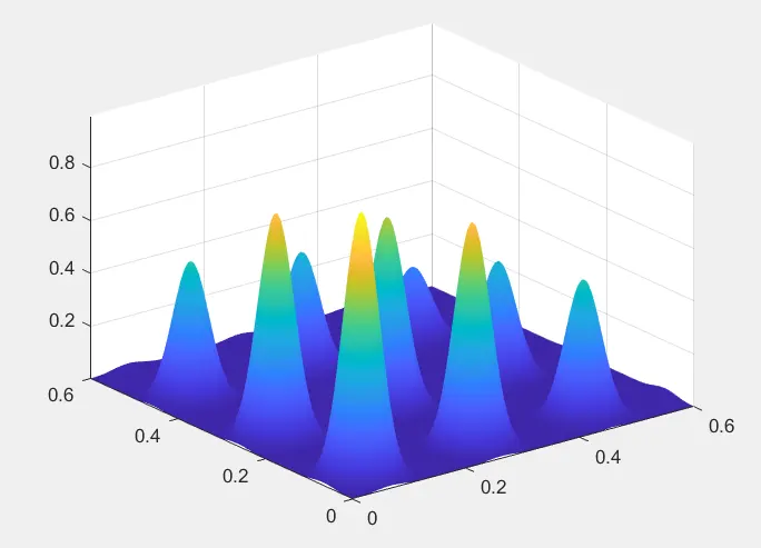
The function creates a 3D plot showing the algorithm
% code for calaculating of the Globel maxima of the Stalagmite function

clear all
close all
clc

%Defining our search space
x=linspace(0,0.6,150);          % Inputs Lower_bound=0; Upper_bound=0.6
y=linspace(0,0.6,150);

%Interaction count

num_cases=50;

tic    % Tic stats the clock time for the enter

%Creating a 2Dmesh
[xx,yy]=meshgrid(x,y);

%Evaluting the stalagmite function
for i=1:length(xx)
    for j=1:length(yy)
        input_vector(1)=xx(i,j);
        input_vector(2)=yy(i,j);
        f(i,j)=Stalagmite(input_vector);
    end
end
Next,we carryout three studies.
1)Unbounded inputs
2)Bounded inputs
3)Bounded inputs with population increased
Unbounded inputs :-
We have No bounds for inputs ,The population is set as a 50,we find the global maximum by giving input as the function and number of design variables .The time taken for this compuiation is calculated by using the tic and toc commands .Then we create a figure window and create a surface plot in it.
% Study-1 Unbounded inputs
tic
for i=1:num_cases
    [inputs,fval(i)]=ga(@Stalagmite,2);
        x_opt(i) = inputs(1);
        y_opt(i) = inputs(2);

end
study1_time =toc;     %Toc stops the timer and Shows the end time

figure(1)
subplot(2,1,1)     % Genarate stalagmite function.
hold on

surfc(x,y,f)
shading interp      % To bring vizually smooth curve surface without mesh lines.


plot3(x_opt,y_opt,fval,'marker','o','markersize',5,'MarkerFaceColor','r')
title('UNBOUNDED INPUTS')
subplot(2,1,2)
plot(fval)
xlabel('interations')
ylabel('Function maximum')
bounded inputs :-
The code is generate the algorithm function built in side the MATLAB.An empty array is created with starting and ending points of the x and y values.
We calculate the global maxima by giving upper and lower bounds along with the function and number of design variables .The population is maintained as 50,As in the previous case ,the time taken to compute is calculated with the help of tic and toc commands .The time is stored in the variable in this study time. Once the global maxima is calculated ,we do the plots as in the previous study, For this study ,we do the plots in a separate figure window.
%Study-2 Bounded inputs

tic
for i = 1:num_cases
    [inputs,fval(i)]=ga(@Stalagmite,2,[],[],[],[],[0,0],[0.3;0.3]);
        x_opt(i) = inputs(1);
        y_opt(i) = inputs(2);

end
study2_time =toc;     %Toc stops the timer and Shows the end time

figure(2)
subplot(2,1,1)     % Genarate stalagmite function.
hold on

surfc(x,y,f)
shading interp      % To bring vizually smooth curve surface without mesh lines.
xlabel('x_values')
ylabel('y_values')
zlabel('z_values')

plot3(x_opt,y_opt,fval,'marker','o','markersize',5,'MarkerFaceColor','b')

title('BOUNDED INPUTS')
subplot(2,1,2)
plot(fval)
xlabel('Number of interations')
ylabel('Function maximum')
Bounded inputs with population increased :-
In this study we calculated the global maxima by giving the same upper and lower bounds but with an increased population .In this case the population set as 200,As in previous studies, the time for computation is calculated using tic and toc commands and stored in the variable study time 3.
For this purpose ,we use the optimizations command .It enables us to change the default population of 50 and implements this population change in the ga.Th plots are plot using the plot command as in previous cases.
%Study -3 Bounded inputs with population increased
options = optimoptions('ga');         %Default values for ga function
options = optimoptions(options,'populationsize',200);  %setting the population size 200

tic
for i = 1:num_cases
    [inputs,fval(i)]=ga(@Stalagmite,2,[],[],[],[],[0,0],[0.3,0.3],[],[],options);
        x_opt(i) = inputs(1);
        y_opt(i) = inputs(2);

end
study3_time =toc;     %Toc stops the timer and Shows the end time

figure(3)
subplot(2,1,1)     % Genarate stalagmite function.
hold on

surfc(x,y,f)
shading interp      % To bring vizually smooth curve surface without mesh lines.


plot3(x_opt,y_opt,fval,'marker','o','markersize',5,'MarkerFaceColor','g');

title('Bounded inputs with population increased')
subplot(2,1,2)
plot(fval)
xlabel('Number of interations')
ylabel('Function maximum')
Main Code (Total):-
% code for calaculating of the Globel maxima of the Stalagmite function

clear all
close all
clc

%Defining our search space
x=linspace(0,0.6,150);          % Inputs Lower_bound=0; Upper_bound=0.6
y=linspace(0,0.6,150);

%Interaction count

num_cases=50;

tic    % Tic stats the clock time for the enter

%Creating a 2Dmesh
[xx,yy]=meshgrid(x,y);

%Evaluting the stalagmite function
for i=1:length(xx)
    for j=1:length(yy)
        input_vector(1)=xx(i,j);
        input_vector(2)=yy(i,j);
        f(i,j)=Stalagmite(input_vector);
    end
end

% Study-1 Unbounded inputs
tic
for i=1:num_cases
    [inputs,fval(i)]=ga(@Stalagmite,2);
        x_opt(i) = inputs(1);
        y_opt(i) = inputs(2);

end
study1_time =toc;     %Toc stops the timer and Shows the end time

figure(1)
subplot(2,1,1)     % Genarate stalagmite function.
hold on

surfc(x,y,-f)
shading interp      % To bring vizually smooth curve surface without mesh lines.


plot3(x_opt,y_opt,-fval,'marker','o','markersize',5,'MarkerFaceColor','r')
title('UNBOUNDED INPUTS')
subplot(2,1,2)
plot(-fval)
xlabel('interations')
ylabel('Function maximum')

%Study-2 Bounded inputs

tic
for i = 1:num_cases
    [inputs,fval(i)]=ga(@Stalagmite,2,[],[],[],[],[0,0],[0.3;0.3]);
        x_opt(i) = inputs(1);
        y_opt(i) = inputs(2);

end
study2_time =toc;     %Toc stops the timer and Shows the end time

figure(2)
subplot(2,1,1)     % Genarate stalagmite function.
hold on

surfc(x,y,-f)
shading interp      % To bring vizually smooth curve surface without mesh lines.
xlabel('x_values')
ylabel('y_values')
zlabel('z_values')

plot3(x_opt,y_opt,-fval,'marker','o','markersize',5,'MarkerFaceColor','b')

title('BOUNDED INPUTS')
subplot(2,1,2)
plot(-fval)
xlabel('Number of interations')
ylabel('Function maximum')

%Study -3 Bounded inputs with population increased
options = optimoptions('ga');         %Default values for ga function
options = optimoptions(options,'populationsize',200);  %setting the population size 200

tic
for i = 1:num_cases
    [inputs,fval(i)]=ga(@Stalagmite,2,[],[],[],[],[0,0],[0.3,0.3],[],[],options);
        x_opt(i) = inputs(1);
        y_opt(i) = inputs(2);

end
study3_time =toc;     %Toc stops the timer and Shows the end time

figure(3)
subplot(2,1,1)     % Genarate stalagmite function.
hold on

surfc(x,y,-f)
shading interp      % To bring vizually smooth curve surface without mesh lines.


plot3(x_opt,y_opt,-fval,'marker','o','markersize',5,'MarkerFaceColor','g');

title('Bounded inputs with population increased')
subplot(2,1,2)
plot(-fval)
xlabel('Number of interations')
ylabel('Function maximum')
Errors -
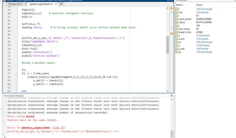
i rectified to change the input vector 'fval' insted of 'f'
Output Plots -
stalagmite function-
Unbounded inputs :-
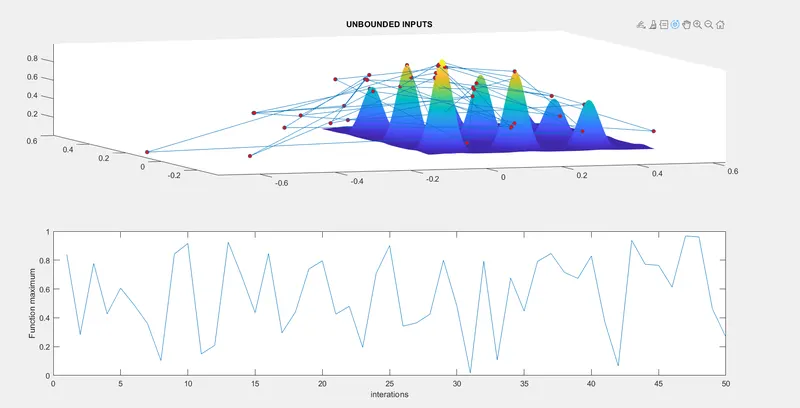
Study time - 6.1679
Bunded inputs :-
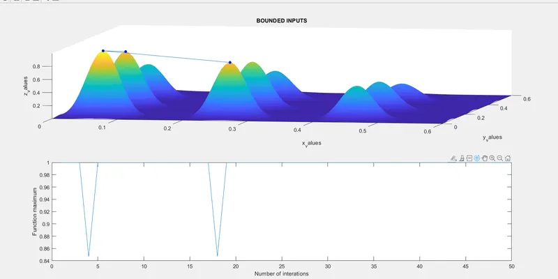
Study time - 7.4509
Bounded inputs with population increased :-
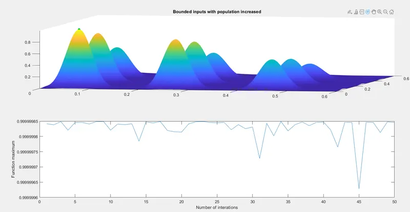
Study time -18.8119
References -
Genetic Algorithm - MATLAB & Simulink (mathworks.com)
https://www.tutorialspoint.com/index.htm