Week 4.1 - Genetic Algorithm

Aim: To write a code in MATLAB to optimize the stalagmite function and find the global maxima of the function.

Objectives:

• Understanding the concept of genetic algorithm.
• Understanding concept of Stalagmite function
• Making use of ‘ga’ function of Matlab to find global maxima of Stalagmite function.
• Plot all the graphs and subplots for each study.

Theory:

Genetic algorithm:

Genetic algorithm is based on the phenomenon of natural selection where fittest individuals are selected for reproduction in order to produce the offspring of next generation. Genetic algorithm repeatedly modifies a population of individual solutions. At each step, the genetic algorithm selects individuals at random from the current population to be parents and uses them to produce the children for the next generation. Over successive generations, the population "evolves" toward an optimal solution. Genetic algorithms are commonly used to generate high-quality solutions to optimization and search problems by relying on biologically inspired operators such as mutation, crossover and selection.

Stalagmite Function:

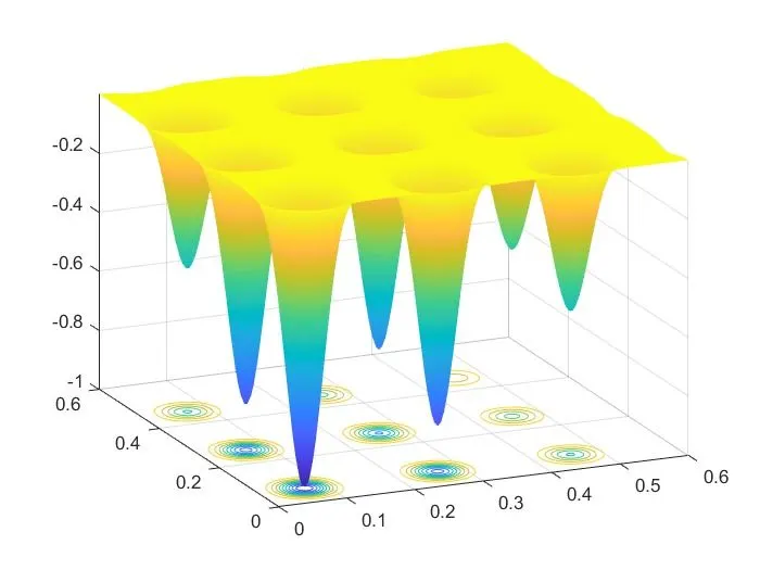
A stalagmite function generally refers to the function with which we are generating values over a stalagmite kind of surface for finding out the local and global maxima and minima of that particular given function.

Genetic algorithm (‘ga’ in Matlab):

ga(fun, nvars, A, b, Aeq, beq, lB, uB, nonlcon, Intcon, options)

fun = objective function
nvars = number of variables
A and b = subject to linear inequalities of the form A*x <=b
Aeq and beq = subject to linear equalities of the form A*x = b
lB = lower bound and uB = upper bound
nonlcon = non-linear inequalities
Intcon = integer constrained
options = helps to add constraint tolerance by increasing the population size.

ProgramCode :-

1) Function Code -

function f_x_y = stalagmite(input_vector)
x = input_vector(1);
y = input_vector(2);
f_1_x = [sin(5.1*pi*x + 0.5)].^6;
f_2_x = exp(-4*log(2)*[x - 0.0667].^2/0.64);
f_1_y = [sin(5.1*pi*y + 0.5)].^6;
f_2_y = exp(-4*log(2)*[y - 0.0667].^2 / 0.64);
f_x_y = -f_1_x * f_2_x * f_1_y * f_2_y;
end

2) Main code -

clc
close all
clear all

%defining our search space
x = linspace(0, 0.6, 150);
y = linspace(0, 0.6, 150);

[xx, yy] = meshgrid(x, y);  %define variables on whole plane

%evaluating the stalagmite function
for i = 1:length(xx)
    for j = 1:length(yy)
        input_vector(1) = xx(i,j);   %saves value of xx according to 'i' and 'j' iteration in 'input_vector'
        input_vector(2) = yy(i,j);   %saves value of yy according to 'i' and 'j' iteration in 'input_vector'
        f(i,j) = stalagmite(input_vector); %find value of 'f' according to 'i' and 'j' iteration
    end
end



num_cases = 50;   % ga will be executed for 50 times
%study 1 (Unbounded)
tic
for i = [1:num_cases]
[inputs fout] = ga(@stalagmite, 2) ; %executing genetic algorithm stating function name and number of variables
xout1(i) = inputs(1);    %storing values of x
yout1(i) = inputs(2);    %storing values of y
fmax1(i) = fout;         %storing values of f
end
study_time1 = toc    %measures time to complete process

figure(1)
subplot(2, 1, 1);    %divides figure window in 2 rows and 1 column and selects 1st row
hold on
surfc(xx, yy, f)  %plots stalagmite function in 3D plot
shading interp   %removes gridlines and provides color shading
xlabel('X Value')
ylabel('Y value')
hold on
plot3(xout1, yout1, fmax1, 'marker', 'o', 'markersize', 5, 'markerfacecolor', 'g')
title('Unbounded Inputs')
hold off
subplot(2,1,2); %select second row of figure window
plot(fmax1);
xlabel('iterations');
ylabel('Maxima')

%study 2  (introducing bounds)
tic
for i = [1:num_cases]
[inputs fout] = ga(@stalagmite, 2, [], [], [], [], [0 0], [0.6 0.6]) ;  %here upper and lower bounds are stated
xout2(i) = inputs(1);
yout2(i) = inputs(2);
fmax2(i) = fout;
end
study_time2 = toc
figure(2)
subplot(2, 1, 1);
hold on
surfc(xx, yy, f)  %plots stalagmite function in 3D plot
shading interp   %removes gridlines and provides color shading
xlabel('X Value')
ylabel('Y value')
hold on
plot3(xout2, yout2, fmax2, 'marker', 'o', 'markersize', 5, 'markerfacecolor', 'g')
title('Bounded Inputs')
hold off
subplot(2,1,2);
plot(fmax2);
xlabel('iterations');
ylabel('Maxima')

%study 3 (Introducing bounds and increasing population size)
tic
%options = optimoptions('ga')
options = optimoptions('ga', 'PopulationSize', 170) %changes PopulationSize to 170
for i = [1:num_cases]
[inputs fout] = ga(@stalagmite, 2, [], [], [], [], [0 0], [0.6 0.6], [], [], options) ; %changed population size is included
xout3(i) = inputs(1);
yout3(i) = inputs(2);
fmax3(i) = fout;
end
study_time3 = toc
figure(3)
subplot(2, 1, 1);
hold on
surfc(xx, yy, f)  %plots stalagmite function in 3D plot
shading interp   %removes gridlines and provides color shading
xlabel('X Value')
ylabel('Y value')
hold on
plot3(xout3, yout3, fmax3, 'marker', 'o', 'markersize', 5, 'markerfacecolor', 'g')
title('Bounded Inputs with increased poulation size')
hold off
subplot(2,1,2);
plot(fmax3);
xlabel('iterations');
ylabel('Maxima')
FMAX3 = -[fmax3];   %converting to global maxima

Explanation :-

First x and y arrays are form having 150 values between 0 to 0.6. Then we convert these arrays into matrix form to have 2 dimensional values to plot a surface graph using ‘meshgrid’ command.

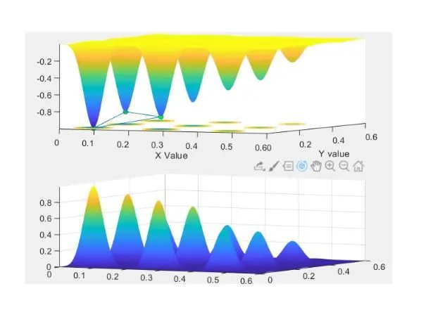
We have created the separate function file for given problem statement and function file name is "stalagmite". In this we have used the formulas(f_x_1,f_x_2,f_x_3,f_x_4) and then multiplied it with each other. Here we use negative sign (-) in function so as to calculate the global maxima.

For study 1, we will use the for loop to run the ‘ga’ function for 50 times. While executing ‘ga’, we specify function name (stalagmite) and number of input variables in the stalagmite function (2; which are x and y). Then, the outputs of this function will be stored in variables ‘xout’, ‘yout’ and ‘fmax’ respectively.
Now, we want to plot 2 graphs for representing the data. So, we will use ‘subplot’ command and divide figure window in 2 rows and 1 column. In top portion of figure window, we will plot surface graph of stalagmite function using command ‘surfc’ and provide color shade using ‘shading interp. Along this, we will also plot values of ‘fmax’; so that values of ‘fmax’ are presented on surface plot itself. To get a simple representation of ‘fmax’ values, we plot its values in the 2nd portion of figure window against 50 iterations. We obtain figure as follows:

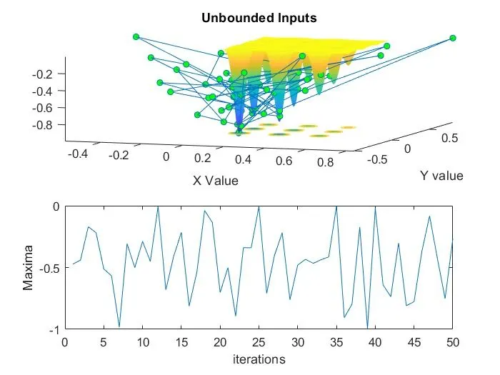
From the above plots, we can observe that values of ‘fmax’ i.e., optimum solution varies too much and hence it is not a stable solution.

To minimize the above problem, we introduce upper and lower bounds in ‘ga’ equation, so that we can narrow down the search area of genetic algorithm so as to get minimum value. The upper and lower bounds for both, ‘x’ and ‘y’ will be 0 and 0.6 respectively. Now, when we execute this part of code, the solution will be found within these input limits only.

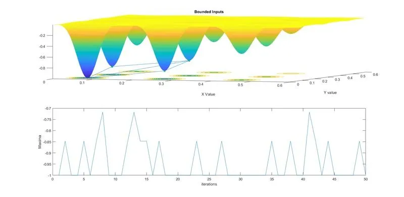
From the above plots, we can observe that values of optimum solution (fmax) are less scattered now and fall under very narrow range.

In genetic algorithm, population size is number of initial inputs, which are a set of ‘x’ and ‘y’ values which are selected according to best fitness results. This population further undergo ‘mutation’ and ‘crossover’ processes to get final optimum solution. If the initial population size is small, code will find local minima; as we see in study 2. So, to find global minima, we have to increase the population size. Default population size of ‘ga’ solver is 50. By using ‘optimoptions’, we replace the default value of ‘PopulationSize’ with 170. Study 3 gives us following results:

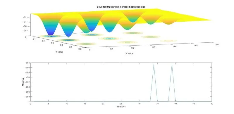
From all the 3 studies and plots, we can observe that ‘ga’ function gave us the global minima, which it the highest point on the highest peak on the whole surface plot. We get the surface plot of stalagmite function in downward direction; on negative side of y-axis because we introduced (-) in function. So, if this negative sign was cancelled, we would get surface plot of same height of peaks on positive side of y-axis. Hence, values of topmost points on upwards and downwards pointing surface plots will be same except for signs. So, in order to get global maxima, we will multiply the global minima we got with (-). Hence, we will get Global maxima using ‘ga’ function in Matlab.

Conclusion :-

• Genetic Algorithm always uses random values and helps to get the best possible outcome with very high accuracy.
• Stalagmite function always gives minima values but for the purpose maxima for the function found to be 1.