Week 3 - Solving second order ODEs

AIM :- To write a program that solves the second order ODE.

OBJECTIVE :-

1. Write a program in Matlab\Octave that will simulate the pendulum motion
2. This ODE represents the equation of motion of a simple pendulum with damping.

INTRODUCTION :-

Simple Pendulum:

A simple pendulum may be described ideally as a point mass suspended by a massless
string from some point about which it is allowed to swing back and forth in a place. A
simple pendulum can be approximated by a small metal sphere which has a small radius
and a large mass when compared relatively to the length and mass of the light string from
which it is suspended. If a pendulum is set in motion so that is swings back and forth, its
motion will be periodic. The time that it takes to make one complete oscillation is
defined as the period T. Another useful quantity used to describe periodic motion is the
frequency of oscillation. The frequency f of the oscillations is the number of oscillations
that occur per unit time and is the inverse of the period, f = 1/T. Similarly, the period is
the inverse of the frequency, T = l/f. The maximum distance that the mass is displaced
from its equilibrium position is defined as the amplitude of the oscillation.

Governing equation:

Second order ODE representing the equation of motion of a simple pendulum motion.

In the above equation,

g = gravity in m/s2,

L = length of the pendulum in m,

m = mass of the ball in kg,

b=damping coefficient.

use,

L=1 metre,

m=1 kg,

b=0.05.

g=9.81 m/s2.

PROGRAM CODE :-

clc
clear all
close all

%inputs
l = 1;     %length_of_pendulam (m)
m = 1;     %mass_ of_ball (kg)
b = 0.05;  %damping_coefficient 
g = 9.81;  %gravity (m/sec^2)

%initial conditions of pendulam
theta_0 = [0; 3];   %displacement = 0 rad, velocity = 3 rad/sec

%timespan
t_span = [0:0.1:20]; %from 0-20 seconds with step size (h) = 0.1

%solving ODE
[t, results] = ode45(@(t, theta) ode_func1(t, theta, b, g, l, m), t_span, theta_0)
  
figure(1)
%plotting graph
plot(t, results(:, 1)); %plots_values_of_1st_column_of_results_ie_angular_displacement
hold on;
plot(t, results(:, 2)); %plots_values_of_2nd_column_of_results_ie_angular_velocity
xlabel('Time');
ylabel('Displacement/Velocity');
grid on;

%creating animation
ct = 1;
angu_disp = results(:, 1);   %storing_values_of_angular_displacement
for i = [1:length(angu_disp)]; 
    THETA = angu_disp(i);
    
    %setting coordnate values of pendulam string
    
    x0 = 0;
    y0 = 0;
    
    x1 = l*sin(THETA);
    y1 = -l*cos(THETA);
    
    figure(2)
   
    plot([-1 1], [0 0],[x0 x1],[y0 y1], 'linewidth', 3); %plotting horizontal line and pendulam string
    hold on;
    %attaching pendulam sphere to string
    plot(x1, y1, 'Marker', 'O', 'MarkerSize', 30, 'MarkerEdgeColor', 'red', 'MarkerFaceColor', [1 0 0]);
    hold off;
    axis([-1.5 1.5 -1.5 1.5]);
    pause(0.08);
    
     %saving_individual_frame
        M(ct) = getframe(gcf);      %save_each_figure_of_graph_as_a_frame
        ct = ct + 1;
    

end

PROGRAM CODE OF FUNCTION "ode.m" :-

function [dtheta_dt] = ode_func1(t, theta, b, g, l, m)
theta1 = theta(1);
theta2 = theta(2);
dtheta1_dt = theta2;
dtheta2_dt = -[b/m]*theta2 - [g/l]*sin(theta1);
dtheta_dt = [dtheta1_dt; dtheta2_dt];   

end

Explanation :-

• Clear all, close all, clc are used to clear the workspace, to clear the graphs that's exist and clar the command window.
• The inputs are mentioned above.
• ode45 is a function in MATLAB that solves ordinary or partial D.E. using a numerical method. In this program the highest order is 2. So, we have to take two constant values to change the equation into simple D.E.
• This function should take at least 2 inputs to solve the equation to the approx. results.
• The ode45 function has a syntax in which we need to specify which should be 't' and 'y' and a timespan for the function to work .
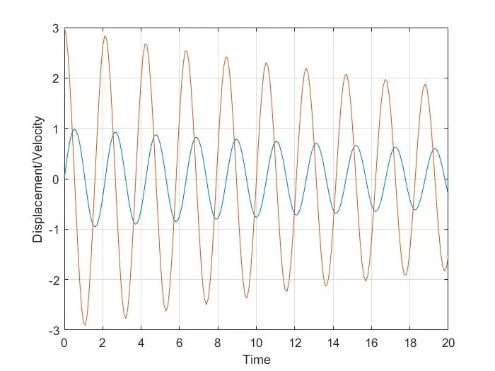
• Figure preswent in result tells how the damping is done for the pendulum. The angular velocity and displacement will cometo rest at the end of the function.
• Those values are plotted by using plot command.
• The label command is used to label the X & Y axis.
• To animate the motion of simple pendulum, a for loop is used to create the specified set of points to keep the bob at different locations.
• x0 and y0 be the fixed point at one end of the string and x1 and y1 be the different position of the bob.
• At each and every point of the bob the 'ct' command which is used to count each and every position and stores the data.
• in the function code, we need to specify the derivatives of theta and the equations to be solved.

RESULT :-

https://drive.google.com/file/d/1fC3ta0z7VVsiOAcQXaCB64QVobzaGKbs/view?usp=drivesdk

Conclusion :-

• We have animated the simple pendulum using the ode45 solver where the second is reduced to a simple differential equation where it is easy to solve the given equation.
• The animation is made using the different points of the bob and the motion of the simple pendulum is used.