Week 4.1 - Genetic Algorithm

Title - Optimise the stalagmite function and find the global maxima of the function.

Aim - 1. Write a code in MATLAB to optimise the stalagmite function and find the global maxima of the function.

2. Plot graphs for all 3 studies and for F maximum vs no. of iterations. Title and axes labels are a must, legends could be shown if necessary.

Code -

Function -

function f = stalagmite(input_vector)

x = input_vector(1);
y = input_vector(2);

f1 = [sin(5.1*pi*x+0.5)].^6;
f2 = [sin(5.1*pi*y+0.5)].^6;
f3 = exp(-4*log(2)*[x-0.0667].^2/0.64);
f4 = exp(-4*log(2)*[y-0.0667].^2/0.64);

f = -(f1*f2*f3*f4);
end

Explaination - This is formula used for finding out minima and as ga only finds the minima,we have used the minus sign.

Main function -

% Defining our search space
x=linspace(0,0.6,150);
y=linspace(0,0.6,150);

num_cases=50; % To run the ga 50 times

[X,Y]=meshgrid(x,y)

% Evaluating the stalagmite function
for i=1:length(X)
    for j=1:length(Y)
        input_vector(1)= X(i,j);
        input_vector(2)= Y(i,j);
        f(i,j)=stalagmite(input_vector); 
% stalagmite function takes in the data given inside parantheses and calculates f
    end
end
surfc(X,Y,f);
xlabel('X axis')
ylabel('Y axis')
shading interp

tic
% Study 1 - Unbounded Condition
for i=1:num_cases
    [inputs,fopt(i)]=ga(@stalagmite,2);

    % ga is an in-built function
    % @ defines what function to minimise
    % ga always minimises a function 
    % 2 denotes the no. of variables in the function, here it is x and y

    xopt(i)=inputs(1);
    yopt(i)=inputs(2);
end

study1_time = toc; 
% tic toc is used to measure how long it takes to study

figure(1)
subplot(2,1,1) % To have multiple plots inside the same figure window
hold on
surfc(x,y,-f)
shading interp
plot3(xopt,yopt,-fopt,'marker','o','markersize',5,'markerfacecolor','r')
title('Unbounded Inputs')
subplot(2,1,2)
plot(-fopt)
xlabel('Iterations');
ylabel('Function minimum');

tic
% Study 2 - Statistical behaviour - with upper and lower bounds
for i=1:num_cases
    [inputs,fopt(i)]=ga(@stalagmite,2,[],[],[],[],[0;0],[1;1]);
    xopt(i)=inputs(1);
    yopt(i)=inputs(2);
end
study2_time=toc;

figure(2)
subplot(2,1,1)
hold on
surfc(x,y,-f)
shading interp
plot3(xopt,yopt,-fopt,'marker','o','markersize',5,'markerfacecolor','r')
title('Bounded Inputs')
subplot(2,1,2)
plot(-fopt)
xlabel('Iterations');
ylabel('Function minimum');

% Study 3 - Increasing GA Iterations
options=optimoptions('ga')
options=optimoptions(options,'PopulationSize',300);

tic
for i=1:num_cases
    [inputs,fopt(i)]=ga(@stalagmite,2,[],[],[],[],[0;0],[1;1],[],[],options);
    xopt(i)=inputs(1);
    yopt(i)=inputs(2);
end
study3_time=toc;

figure(3)
subplot(2,1,1)
hold on
surfc(x,y,-f)
shading interp
plot3(xopt,yopt,-fopt,'marker','o','markersize',5,'markerfacecolor','r')
title('Bounded Inputs with Modified Population Size')
subplot(2,1,2)
plot(-fopt)
xlabel('Iterations');
ylabel('Function minimum');

study 1- unbounded bonds - here no bounds are set and hence the points vary along a wast area of plane.

Results for study 1 -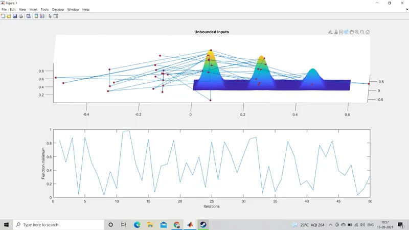

Study 2 - by setting the lower and upper bounds - by setting this we get a local maxima

Results of study 2 -

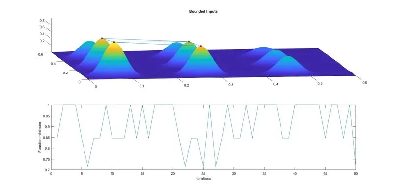
study 3 - here we increase the number of itirations or populations by 300

Results of study 3 -

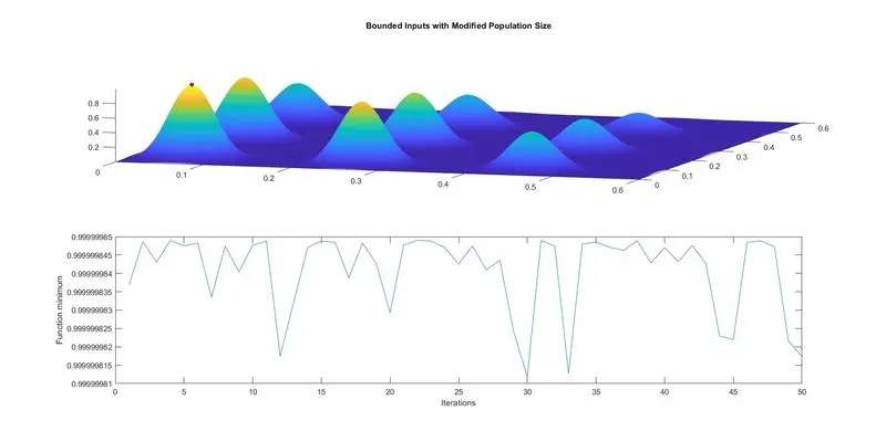
Conclusion - Hence a global Maxima was calulated using the ga.