Week 4.1 - Genetic Algorithm
Aim : A code in MATLAB to optimise the stalagmite function and find the global maxima of the function.
Theroy:
A genetic algorithm (GA) is a method for solving both constrained and unconstrained optimization problems based on a natural selection process that mimics biological evolution. The algorithm repeatedly modifies a population of individual solutions. At each step, the genetic algorithm randomly selects individuals from the current population and uses them as parents to produce the children for the next generation. Over successive generations, the population "evolves" toward an optimal solution.
You can apply the genetic algorithm to solve problems that are not well suited for standard optimization algorithms, including problems in which the objective function is discontinuous, nondifferentiable, stochastic, or highly nonlinear.
Five phases are considered in a genetic algorithm.
- Initial population
- Fitness function
- Selection
- Crossover
- Mutation
Initial Population
The process begins with a set of individuals which is called a Population. Each individual is a solution to the problem you want to solve.
Fitness funtion
The fitness function determines how fit an individual is (the ability of an individual to compete with other individuals). It gives a fitness score to each individual. The probability that an individual will be selected for reproduction is based on its fitness score.
Selection
Two pairs of individuals (parents) are selected based on their fitness scores. Individuals with high fitness have more chance to be selected for reproduction
Crossover
Crossover is the most significant phase in a genetic algorithm. For each pair of parents to be mated, a crossover point is chosen at random from within the genes.
Mutation
In certain new offspring formed, some of their genes can be subjected to a mutation with a low random probability. This implies that some of the bits in the bit string can be flipped.
Function Code:
function [f]=stalagmite(input_vector)
x = input_vector(1);
y = input_vector(2);
f1=(sin(5.1*pi*x+0.5)).^6;
f2=(sin(5.1*pi*y+0.5)).^6;
f3=exp(-4*log(2)*(x-0.0667).^2/0.64);
f4=exp(-4*log(2)*(y-0.0667).^2/0.64);
f= -f1*f2*f3*f4;
end
At the end of the function we are using -ve sign ,as we have to find the maxima of the function of ga.
Syntax fo ga:
close all
clc

%defining our search space
x = linspace(0,0.6,150);
y = linspace(0,0.6,150);
[x,y]=meshgrid(x,y);
num_case=50;

for i=1:length(x)
    for j=1:length(y)
        input_vector(1)=x(i,j);
        input_vector(2)=y(i,j);
f(i,j) = stalagmite(input_vector);
    end
end
 surfc(x,y,f);
 shading interp

%study-1 statistical behavior
tic
for i=1:num_case
    [input,fopt(i)] = ga(@stalagmite,2);
    xopt(i) = input(1);
    yopt(i) = input(2);
end

study_time_1 = toc
figure(1)
subplot(2,1,1);
hold on
surfc(x, y, -f);
shading interp
plot3(xopt,yopt,-fopt,'marker','o','markersize',5,'markerfacecolor','r')
title('unbounded inputs')
subplot(2,1,2)
plot(-fopt)
xlabel('iteration')
ylabel('function minimum')

%study - 2 - statistical behavior with upper and lower bounds
tic
for i =1:num_case
    [input,fopt(i)] = ga(@stalagmite,2,[],[],[],[],[0;0],[1;1]);
    xopt(i) = input(1);
    yopt(i) = input(2);
end
toc
figure(2)
subplot(2,1,1)
hold on
surfc(x,y,-f)
shading interp
plot3(xopt,yopt,-fopt,'marker','o','markersize',5,'markerfacecolor','r');
subplot(2,1,2)
plot(-fopt)
xlabel('iteration')
ylabel('function minimum')


%study 3 increasing the ga iterations
options = optimoptions('ga');
options = optimoptions(options,'populationSize',200);
tic
for i=1:num_case
    [input,fopt(i)]=ga(@stalagmite,2,[],[],[],[],[0;0],[1;1],[],[],options);
    xopt(i)=input(1);
    yopt(i)=input(2);
end
toc
figure(3)
subplot(2,1,1)
hold on
surfc(x,y,-f)
shading interp
plot3(xopt,yopt,-fopt,'marker','o','markersize',5,'markerfacecolor','r');
title('bounded input')
subplot(2,1,2)
plot(-fopt)
xlabel('iteration')
ylabel('function minimum')
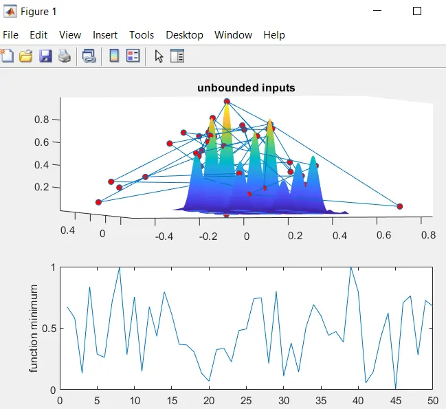
Results for Study -1 Statistical behavior:
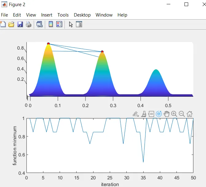
Results for study -2 statistical behavior with lower and upper bound:
Results for study -3 Increasing ga Iteration:
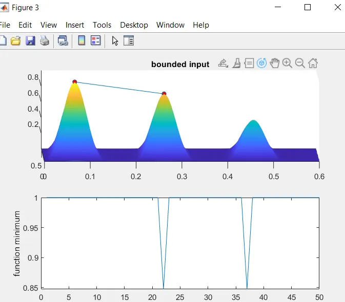
As we increase the number of iteration the time for the results also increases.