Week 3 - Solving second order ODEs

Aim:Write a program in Matlab that will simulate the pendulum motion using Second order ODE.

Theory:

The simple pendulum is another mechanical system that moves in an oscillatory motion. It consists of a point mass ‘m’ suspended by means of light inextensible string of length L from a fixed support as shown.

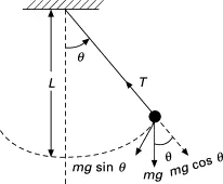
In Engineering, ODE is used to describe the transient behavior of a system. The way the pendulum moves depends on the Newtons second law. When this law is written down, we get a second order Ordinary Differential Equation that describes the position of the "ball" w.r.t time.

This ODE represents the equation of motion of a simple pendulum with damping

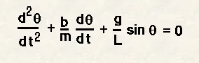
In the above equation,

g = gravity in m/s2,

L = length of the pendulum in m,

m = mass of the ball in kg,

b=damping coefficient.

Fixed Parameters:

L=1 metre,

m=1 kg,

b=0.05.

g=9.81 m/s2

Here,

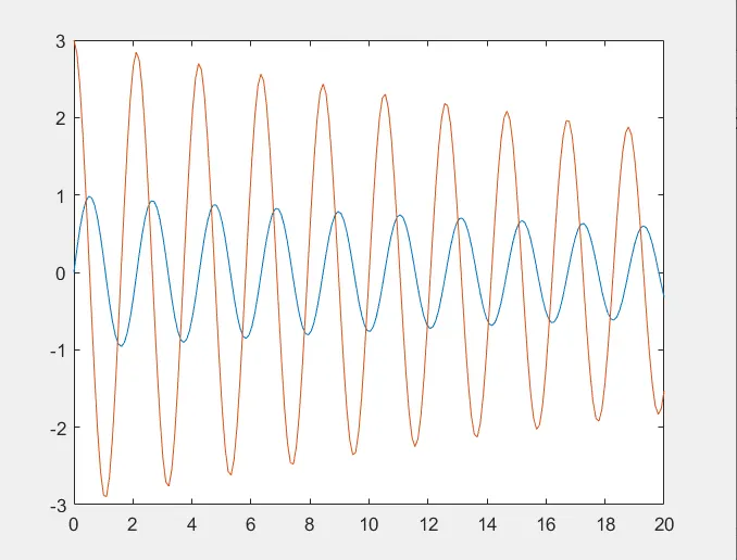
We are Simulating the motion between 0-20 sec, for angular displacement=0,angular velocity=3 rad/sec at time t=0.

Code:

ODE function code:

function[dtheta_dt]=ode_func(t,theta,b,g,l,m)

theta1=theta(1)
theta2=theta(2)
dtheta1_dt=theta2;
dtheta2_dt=-(b/m)*theta2-(g/l)*sin(theta1);
dtheta_dt=[dtheta1_dt;dtheta2_dt];
end

Explanation:

1) In this code the Second order ODE is Simplified into first order ODE, by introducing the terms theta1 and theta2.

2)Here the function declare ode function for t, theta, b, g,l,m.

3)Then this theta1 and theta2 are diffrentiated and dtheta_dt gives a column Matrix.

Main code:

clear all
close all
clc

b=0.05;
g=9.81;
l=1;
m=1;
%initial condition
theta_0=[0;3];

%timepoints 
t_span=linspace(0,20,200)

%solve ODE
[t,result]=ode45(@(t,theta)ode_func(t,theta,b,g,l,m),t_span,theta_0);

plot(t,result(:,1))
hold on 
plot(t,result(:,2))

ct=1;
for i=1:length(result(:,1))                    
    x0=0;
    y0=0;

x1=l*sin(result(i,1));
y1=-l*cos(result(i,1));

figure(2)
%plotting 
plot([x0 x1],[y0 y1],'linewidth',3)
axis([-2 2 -2 2])
hold on
plot([-1 1],[0 0],'linewidth',4)

plot(x1,y1,'.','MarkerSize',30)

M(ct)= getframe(gcf);   
ct= ct+1;
hold off

end
    movie(M)
    videofile=VideoWriter('ode_function_for_loop.avi','uncompressed AVI');
    open(videofile)
    writeVideo(videofile,M)
    close(videofile)

Explanation:

1)First in the Editor window the parameters for b,g,l,m are given

2)Here the theta_0 represents angular displacement i.e is 0 and angular velocity i.e 3 rad/sec.

3)In the t_span 200 values are taken between 0 to 20 time period .

4)Now Using ODE 45 Command ODE function is given.

5)Now using plot Command angular displacement and angular velocity is plotted.

6)Now we are using for loop command as 'i' i.e for angular displacement.

7)For plotting the bob we are using point i.e '.' and increasing size by MarkerSize upto 30.

8)Using the Movie Command the plot are saved in uncompressed avi.

Plot Image:

Animation:https://youtu.be/HsC7R8ZhxII

Result:

Here we have Simulated simple pendulum using ODE function.