Week 4.1 - Genetic Algorithm

The Genetic Algorithm

The GA is derived from the process that drives biological evolution. The process of evolution starts by selecting the fittest individuals from a population. They then produce offspring that inherit the properties of their parents and will be called the next generation. If parents have better fittness then their offspring will have a better chance of survival.This iteration keeps going and at the end a generation with the fttest individuals will be found. The algorithm randomly selects the parents for the next generation. Over succesive generations, the population keeps evolving towards a common goal. The genetic algorithm can be applied to a variety of optimisation problems in which standard optimisation tecniques cannot be used.

The GA uses 3 main types of rules to create the next generation:

• Selection Rules, select the individuals that contributes towards the next generations (parents)
• Crossover rules, combine two parents to form children.
• Mutation Rules, apply random changes to individual parents to form children.

The algorithm does the following steps:

• Creates random initial population
• Scales the raw fittness scores to convert them into more usable range of values. These scaled values are called expectation values.
• Then it selects members called parents based on their expectation.
• Along with the individuals that has high fitness values, some individuals in the current population that have lower fitnessess are chosen as elite. These elite individuals are passed to the next population. Also it produces children by making random changes to a single parent called mutation or by combining the vector entries of a pair of parents called crossover.
• It then replaces the current population to form children to form next generation.
• Then it scores each member of the current population by computing the fitness values. These values are called raw fitness scores.

The algorithm stops when one of the stopping criteria is met.

Main Code:

clear all 
close all
clc
x = linspace(0,0.6,150);
y = linspace(0,0.6,150);
num_cases=50;
%Creating a 2D mesh
[xx yy] = meshgrid(x,y);
%Evaluvating Stalgamite Function
for i = 1:length(xx);
    for j = 1:length(yy);
        input_value(1)= xx(i,j);
        input_value(2)= yy(i,j);
        f(i,j) = stalgamite(input_value);
    end
end

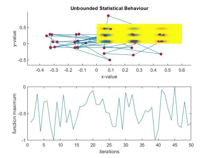
%Unbounded statistical behaviour
tic
for i=1:num_cases;
    [inputs1,fopt1(i)]=ga(@stalgamite,2);
     xopt(i)=inputs1(1);
     yopt(i)=inputs1(2);
end 
study1_time=toc;
figure(1)
subplot(2,1,1)
hold on
surfc(xx,yy,f)
xlabel('x-value')
ylabel('y-value')
zlabel('function value')
shading interp
plot3(xopt,yopt,fopt1,'marker','o','markersize',5,'markerfacecolor','r')
title('Unbounded Statistical Behaviour')
subplot(2,1,2)
plot(fopt1)
xlabel('iterations')
ylabel('function maximum')
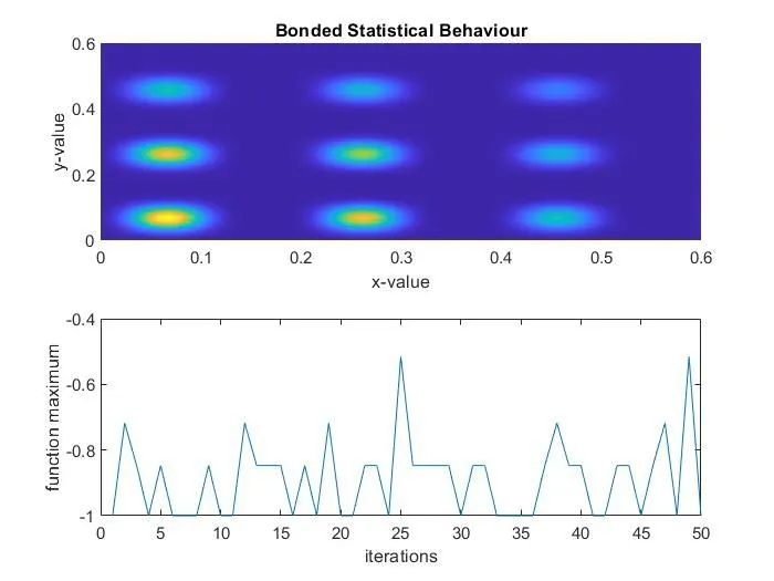
%Statistical Behaviour with Upper and lower bound
tic;
for i=1:num_cases;
    [inputs2,fopt2(i)]=ga(@stalgamite,2,[],[],[],[],[0;0],[1;1]);
    xopt(i)=inputs2(1);
    yopt(i)=inputs2(1);
end
study2_time=toc;
figure(2)
subplot(2,1,1)
hold on
surfc(xx,yy,-f)
xlabel('x-value')
ylabel('y-value')
zlabel('function value')
shading interp
plot3(xopt,yopt,fopt2,'marker','o','markersize',5,'markerfacecolor','r')
title('Bonded Statistical Behaviour')
subplot(2,1,2)
plot(fopt2)
xlabel('iterations')
ylabel('function maximum')

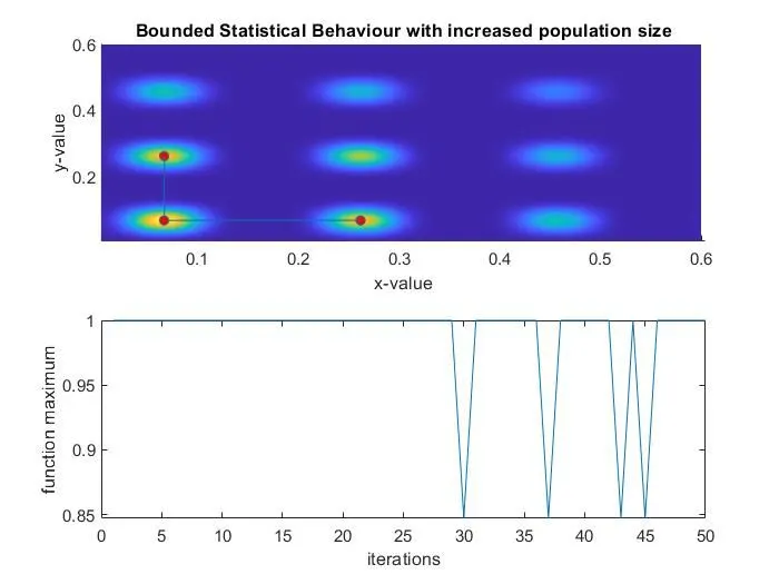
%Increasing GA Population Size
options=optimoptions('ga');
options=optimoptions(options,'populationsize',170);
tic
for i=1:num_cases;
    [inputs3,fopt3(i)]=ga(@stalgamite,2,[],[],[],[],[0;0],[1;1],[],[],options);
    xopt(i)=inputs3(1);
    yopt(i)=inputs3(2);
end
study3_time=toc;
figure(3)
subplot(2,1,1)
hold on
surfc(xx,yy,-f)
xlabel('x-value')
ylabel('y-value')
zlabel('function value')
shading interp
plot3(xopt,yopt,-fopt3,'marker','o','markersize',5,'markerfacecolor','r')
title('Bounded Statistical Behaviour with increased population size')
subplot(2,1,2)
plot(-fopt3)
xlabel('iterations')
ylabel('function maximum')
Total_time=study1_time+study2_time+study3_time
fprintf('n The results are below:')

fprintf('nn Study 1: Unbounded Statistical Behaviour')
fprintf('nn The time taken for study 1 is :%f',study1_time)
fprintf('n The co-ordinates of x and y for global maxima of the funtion are: %f %f',inputs1(1),inputs1(2))
fprintf('nn The Global maxima of the function is :%f',-(mean(fopt1)))

fprintf('nn Study 2: Unbounded Statistical Behaviour')
fprintf('nn The time taken for study 2 is :%f',study1_time)
fprintf('n The co-ordinates of x and y for global maxima of the funtion are: %f %f',inputs2(1),inputs2(2))
fprintf('nn The Global maxima of the function is :%f',-(mean(fopt2)))

fprintf('nn Study 3: Unbounded Statistical Behaviour')
fprintf('nn The time taken for study 3 is :%f',study1_time)
fprintf('n The co-ordinates of x and y for global maxima of the funtion are: %f %f',inputs3(1),inputs3(2))
fprintf('nn The Global maxima of the function is :%f',-(mean(fopt3)))

Explanation:

1. Linespace command is used to define x and y with 150 elements between 0 and 0.6 including the bounds.
2. Then a 2D grid is made using mesh grid command.
3. For loop is used to solve the GA for every element in the 2D mesh grid.
4. The length of rows and colomns are used as counters.
5. The input vector is declared and GA requires input vector which is each value in mesh grid.
6. The output of stalgamite function is stored in matrix.
7. Tic command is used to start timer
8. For loop bounded by number of iterations is formed.
9. GA code is entered for the unbounded statistical study
10. The minimum value of the funtion for each value is outputed and its x and y coordinates are stored in seperate variables.
11. The toc command is used to stop the timer and output is stored in study_time1.
12. Next the figure 1 is plotted
13. Subplot command is used to partition the window in order to draw more than one plot in the same window.
14. Hold command is used to prevent plot from being removed.
15. The surfc command is used to plot contour with xx value and yy value from the mesh grid as input, negative optimum value is used because we need to maximize the functon
16. X, y and Z axis are labled.
17. Shading intrep is used to smoothen the function plot and remove the grid lines.
18. Plot 3 command is used to plot a point in 3 dimensions. Here it will plot -fopt because we need the maximum value of the function.
19. Graph title is entered.
20. -Fopt value is plotted on the second plot in second row.
21. The same study is made but this time it is bounded. (has upper and lower limit)
22. The range of the GA is bounded by introducing values in lower and upper bounds and hence the values of maxima and the values of x and y will be within the defined space in inputs.
23. Then increasing population study was done
24. Total time is computed.
25. Results are printed in the command window

Stalgamite Function code:

function [f] = stalgamite(input_value)

f_1_x =(sin(5.1*pi*input_value(1) + 0.5))^6;
f_1_y =(sin(5.1*pi*input_value(2) + 0.5))^6;
f_2_x = exp(-4*log(2)*(((input_value(1)-0.0667)^2)/(0.64)));
f_2_y = exp(-4*log(2)*(((input_value(2)-0.0667)^2)/(0.64)));

f=(-f_1_x*f_1_y*f_2_x*f_2_y);
end

RESULTS