Week 4.1 - Genetic Algorithm

Objective Of the Project :

1. Explaining the concept of generic algorithm and also explain the syntax for ga in matlab.
2. plot the graphs for all 3 studies and fr F maximum vs No of iterations.

Introduction:

In computer science and operations research, a genetic algorithm (GA) is a metaheuristic inspired by the process of natural selection that belongs to the larger class of evolutionary algorithms (EA). Genetic algorithms are commonly used to generate high-quality solutions to optimization and search problems by relying on biologically inspired operators such as mutation, crossover and selection.

The genetic algorithm is a technique for solving both constrained and unconstrained optimization problems that are based on natural selection, the process that drives biological evolution. The genetic algorithm constantly modifies the population size of individual solutions.

Phases in Generic Algorithm :

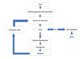
1. Initialization of population(coding)

The code generates random population of a defined size and from that the code evaluates the fitness of the members from which the new population can be formed using the iterations.

2.Fitness Function

It is that function which we optimize and the optimization process i done with the help of number of generations formed by the code with respect to the fitness value of each number.

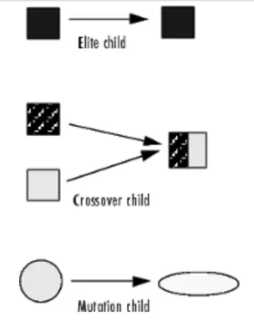
3. Selection phase

In the selection phase there are various methods like

1.crossover

2.mutation

from which the ga tries to select the fittest individual.

GA SYNTAX

x = ga (fun,nvars)

x = ga(fun,nvars,A,b)

x = ga(fun,nvars,A,b,Aeq,beq)

x = ga(fun,nvars,A,b,Aeq,beq,lb,ub)

x = ga(fun,nvars,A,b,Aeq,beq,lb,ub,nonlcon)

x = ga(fun,nvars,A,b,Aeq,beq,lb,ub,nonlcon,options)

x = ga(fun,nvars,A,b,[],[],lb,ub,nonlcon,IntCon)

x = ga(fun,nvars,A,b,[],[],lb,ub,nonlcon,IntCon,options)

x = ga(problem)

[x,fval] = ga(___)

[x,fval,exitflag,output] = ga(___)

[x,fval,exitflag,output,population,scores] = ga(___)

DESCRIPTION

x=ga(fun,nvars) finds a local unconstrained minimum,x,to the objective function, fun.nvars is the dimension of fun.

x=fa(fun,nvars,A,b) finds a local minimum x to fun,subject to the linear inequalities A*x<=b.ga evaluates the matrix product A*x as if x is transposed (A*x').

x= ga(fun,nvars,A,b,Aeq, beq,lb,ub) defines a set of lower and upper boundaries on the design variables x so that a solution is found between lb and ub ( set Aeq=[] and beq=[] if there is no linear equalities exist .

x = ga(fun,nvars,A,b,Aeq,beq,lb,ub,nonlcon,intcon,options)

requires that the variables listed in intcon take the integer values

x= ga (problem)

finds the minimum for a problem .

[x.fval,exitflag,outout] = ga(___) also returns exitflafan integer identifying the reasom the algorithm terminated, and output, a structure that contains output from each generation and other information about the performance of the algorithm.

stalagmite Equation

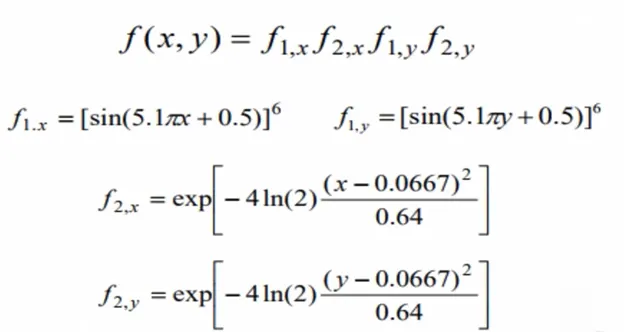
from this equation the function code is derived for the problem

function [f] = stalagmite(input_vector)
x = input_vector(1);
y = input_vector(2);

term1 = (sin((5.1*pi*x)+0.5))^6;
term2 = (sin((5.1*pi*y)+0.5))^6;
term3 = exp(-4*log(2)*((x-0.0667)^2)/0.64);
term4 = exp(-4*log(2)*((y-0.0667)^2)/0.64);



[f]= -(term1*term2*term3*term4);

end

clear all
close all
clc

x = linspace(0,0.6,150)
y = linspace(0,0.6,150)

 %Number of iterations
num_cases = 50 ;


%coverting x and y to matrix by using the command meshgrid
[xx yy] = meshgrid(x,y);

for i=1:length(xx)
for j= 1:length(yy)
    input_vector(1)= xx(i,j);
    input_vector(2)= yy(i,j);
    f(i,j)= stalagmite(input_vector);
end
end

%creates a 3 dimensional surface 
figure(1)
surfc(xx,yy,-f)
shading interp %makes the plot clearer
xlabel('x value')
ylabel('y value')
title('stalagmite function')


% study 1
%statistical behaviour with unbounded limits
tic
for i = 1:num_cases
    [inputs ,fopt(i)]= ga(@stalagmite,2)
    xopt(i) = inputs(1);
    yopt(i) = inputs(2);
end
study_1=toc
figure(2)
subplot(2,1,1)
hold on
surfc(x,y,-f)
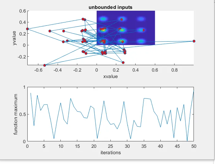
title('unbounded inputs')
xlabel('xvalue')
ylabel('yvalue')
shading interp

hold on 

plot3(xopt,yopt,-fopt,'marker','o','markersize',5,'markerfacecolor','r')
subplot(2,1,2)
plot(-fopt)
xlabel('iterations')
ylabel('function maximum')

%study_2 statistical study with bounded limits

tic
for j = 1:num_cases 
    [inputs,fopt(j)]=  ga(@stalagmite,2,[],[],[],[],[0;0],[0.6;0.6]);
    xopt(j) = inputs(1);
    yopt(j) = inputs(2);
end
study_2_time= toc
figure(3)
subplot(2,1,1)
surfc(x, y, -f);
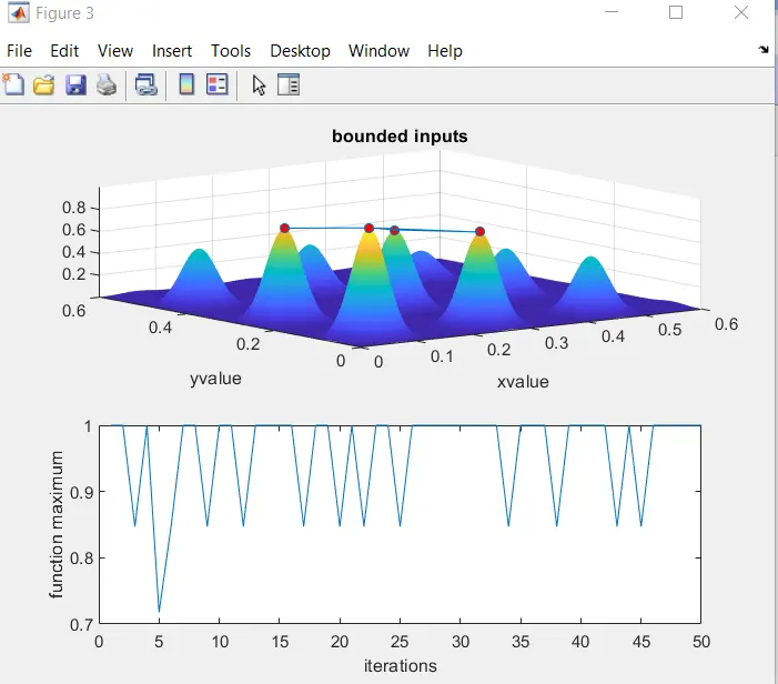
title('bounded inputs')
xlabel('xvalue');
ylabel('yvalue');
shading interp
hold on

plot3(xopt,yopt,-fopt,'marker','o','markersize',5,'markerfacecolor','r')
subplot(2,1,2)
plot(-fopt)
xlabel('iterations')
ylabel('function maximum')

%study 3 statistical study with increasing the number of population by
%using optimoptions command 

options = optimoptions(@ga)
options = optimoptions(@ga,'populationsize',500)

tic
for k = 1:num_cases
    [inputs,fopt(k)] = ga(@stalagmite,2,[],[],[],[],[0;0],[0.6;0.6],[],[],options);
    xopt(k)= inputs(1);
    yopt(k)= inputs(2);
end

study_3_time = toc 
figure(4)

subplot(2,1,1)
surfc(x,y,-f)
xlabel('xvalue')
ylabel('yvalue')
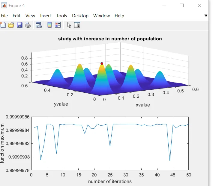
title('study with increase in number of population')
shading interp 

hold on 

plot3(xopt,yopt,-fopt,'marker','o','markersize',5,'markerfacecolor','r');
subplot(2,1,2)
plot(-fopt);
xlabel('number of iterations')
ylabel('function maximum')

figure (1) shows the plot of stalagmite function of the random values .

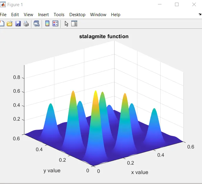
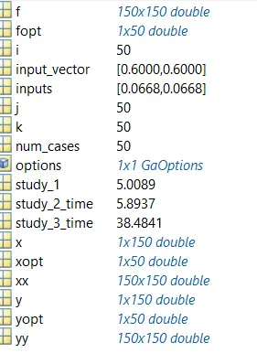
The below figure shows the optimumvalues on different points and we cannot determine the function maximum and time taken for the study 1 5.0089 seconds

study 2 plot shows that the optimum values are limited within the given boundaries in the program and hence its a bit clearer from the previous figure but not yet clear to find the function maximum. To determine the function maximum we should consider the 3rd study with increase in number of population and by using the optimoptions command in the matlab program.

0

In the figure 4 it it clear that markerface points at only one point and that point is nearly 0.999 which is the function maximum approximately.

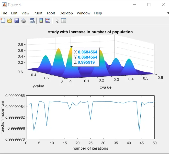
on Rotating this plot we can say that the value of

x = 0.068

y = 0.068

Errors

*No major errors were faced during the coding *

REFERENCES:

https://riadalam323.medium.com/?p=9a4373ffee93

LEAVE A COMMENT: