Week 3 - Solving second order ODEs

AIM :

To create a program solving second order ode and create a pendulum animation

THEORY :

A simple pendulum of string length l and the mass of the ball being m is attached to a rigid link. when the external force acts on in it changing from its equilibrium position to oscillate in a circular motion in a vertical plane .

This motion can be dreived by mathematical expression using the ode functtion in the matlab program thus representing the motion .

Ode is used to describe transient behaviour of the system. such an example is simple pendulum.

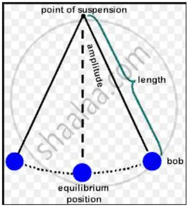
Governing Equation:

The following equation is given as:

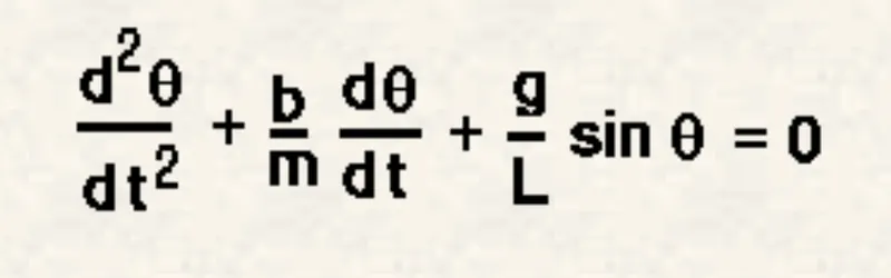
In the above equation

g = 9.81, Acceeleration due to gravity m/s^2

m = 1, mass of the ball in kg

L= 1, length of the pendulum in m

b = 0.05 , damping coefficient .

Procedure :

• In order to solve this firstly the second order equation is converted to first order equation an which then can be used in an ode function
• Now input the values of g m b and l and also give the values for time and the angular displacement.
• Now give the syntax foe the ode function which involves the values of theta, time span, g , b, l , and m
• now plot the results with angular displacement and time .
• give the function of ode

The procedure for pendulum oscillation:

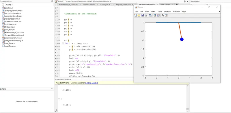
To create and animation firstly the values of x0 y0 x1 y1 x2 y2 is given accordingly and and for function is used to give different values of the results obtained and different values of theta.

Then the lines are plotted using plot command and the movie is created using the movie command and the videowrite and videofile command .

clear all
close all
clc

b=0.05; %damping
g=9.81; %Acceleration due to gravity
l = 1; %length of the string
m= 1 ; % mass in kg

%initial condition
theta_0 = [0;3];

%time points 

t_span = linspace(0,20,100);

%[t,results ]= (challenge_2nd_ode , t_span, theta_0)
[t,results]= ode45(@(t,theta)ode_func(t,theta,b,g,l,m),t_span,theta_0);

plot(t,results(:,1))
hold on
plot(t,results(:,2))
xlabel('time')
ylabel('plot')
title('2nd order ode plot')



%Animation of the Pendulum

x0 = 0
y0 = 0
x1 = -2
y1 = 0
x2 = 2
y2 = 0 

ct = 1
for i = 1:length(t)
    x = l*sin(results(i))
    y = -1*cos(results(i))
    
    plot([x1 x0 x2],[y1 y0 y2],'linewidth',3)
    hold on 
    plot([x0 x],[y0 y],'linewidth',3)
    plot(x,y,'o','markersize',17,'markerfacecolor','b')
    axis([-3 3 -3 0])
    hold off
    pause(0.03)
    d(ct)= getframe(gcf);
    ct= ct + 1
    
end

movie(d)
videofile = VideoWriter('simple_pendulum.avi','uncompressed AVI')
open(videofile)
writeVideo(videofile,d)
close(videofile)

function [dtheta_dt] = ode_func(t,theta,b,g,l,m)
theta1=theta(1)
theta2=theta(2)
dtheta1_dt = theta2
dtheta2_dt = -(b/m)*theta2 -(g/l)*sin(theta1);
dtheta_dt = [dtheta1_dt;dtheta2_dt ];

end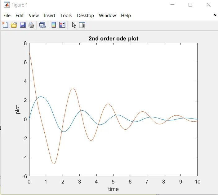

YOUTUBE LINK FOR THE PENDULUM ANIMATION:

https://youtu.be/T8i-Mwj0BTI

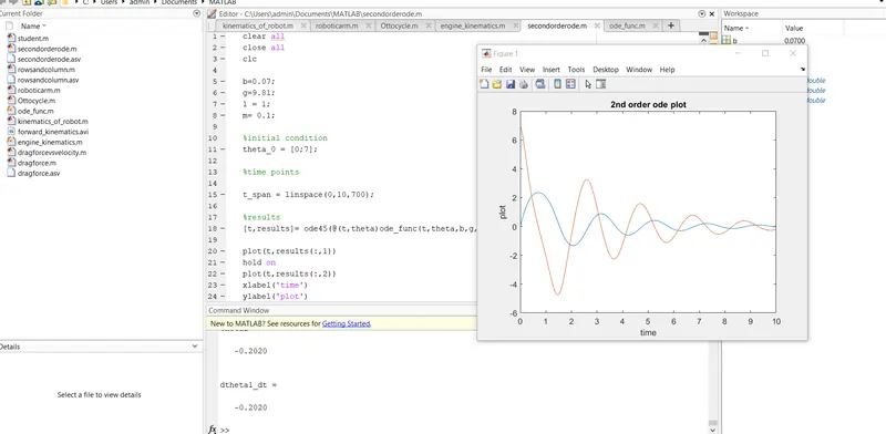
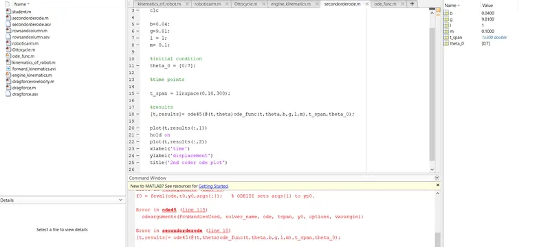
some of the mistakes which i have made in ode sytax is shown above in the screenshot provided.

Conclusion :

Thus the movie of pendulum oscillation is created and and a youtube link is provided. and also we can say that we can reduce or increase the speed of the motion by varying the linspace values .

LEAVE A COMMENT :