Week 4.1 - Genetic Algorithm

Genetic Algorithm:-

An Algorithm is a step-by-step instruction for computers to solve problems. A Genetic Algorithm is an evolutionary algorithm that uses several steps before giving the final best possible value. It is based on evolution in nature. The algorithm creates several random creatures based on the objectives; this creation is known as forming the first generation on the basis of random sampling. It selects the two best parents and produces several offspring from them and simultaneously mutates them. This is done until we don’t get the best results based on certain objectives.

Working (Example):-

1. Assume you need to determine the distance where load can be acted on a cantilever beam to generate less stress.
2. The objective functions here will be the cantilever bending stress equation.
3. The input parameters meters will be the load(W) and length of the point at which load is acting(x,a)
4. An array is generated for both Load and distance within certain limits, 'load' is fixed whereas the distance varies.
5. The Genetic algorithm determines the distance at which least stresses will be generated on the beam and accordingly we can make the load act over there which increase the life-cycle of the cantilever beam.

Genetic algorithm syntax:-

x = ga(fun,nvars,A,b,[],[],lb,ub,nonlcon,IntCon,options)

1.’ga’ is used for calling the genetic algorithm function

2.’fun’ is for determining the function handle we created.

3.’nvars’ for defining the number of variables used in the program(function handle, main handle).

4.‘A,b’ these are linear equality constraints that are subjected to find local minimum x.

5.’lb,ub’ are used to determine the upper limit and lower limits, we expect our results to be in this range.

6.’Options’ It is an optimization option where population size can be changed(increased mostly) in order to get more accurate.

Procedure:-

1. The function is created using the formulas given, it is named as stalagmite which has 2 variables x and y. Since the Ga’s purpose is to find the global Minima we make the function negative in order to generate maxima point.
2. The main Program is written where input arrays are generated.
3. A sample size is determined in this case its 50.
4. Three studies are shown over here. A forloop is created at length of sample size and after feeding in the inputs; the output is generated, although it is not accurate in every case.
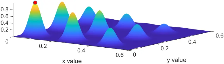
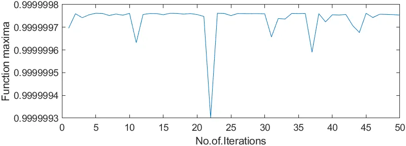
5. After every study graph is plotted, using subplot function, first a 3-d Graph is plotted which showcases the x,y,f which also showcases the maxima output (fopt). Secondly in the plot fopt is individually plotted over the course.
6. In study 1, we just feed the function handle and number of variables in the syntax. This doesn’t give us a single optimum point. Hence it is not reliable.
7. In study 2, along with handle name and variable numbers we also feed the upper and lower boundary limit so that the output is generated only within a required range. This time we see the output is within a limited range although it is still varying.
8. In study 3, we define all the values which were put in first 2 cases, but the sample size over here has been increased in order to get an optimum value which is successfully done here.

function [f] = stalagmite3(input_vector)%function handle for Global maxima
x = input_vector(1);
y = input_vector(2);
f1_x = (sin((5.1*3.14*x)+0.5)).^6;
f1_y = (sin((5.1*3.14*y)+0.5)).^6;
f2_x = exp(-4*log(2)*(x-0.0667).^2/0.64);
f2_y = exp(-4*log(2)*(y-0.0667).^2/0.64);
f = -((f1_x)*(f1_y)*(f2_x)*(f2_y));
end

-----------------------------------------------------------------------------------------
function [f] = stalagmite(input_vector)%function handle for global minima
x = input_vector(1);
y = input_vector(2);
f1_x = (sin((5.1*3.14*x)+0.5)).^6;
f1_y = (sin((5.1*3.14*y)+0.5)).^6;
f2_x = exp(-4*log(2)*(x-0.0667).^2/0.64);
f2_y = exp(-4*log(2)*(y-0.0667).^2/0.64);
f = (f1_x)*(f1_y)*(f2_x)*(f2_y);
end

-----------------------------------------------------------------------------------------
clear all
close all
clc

%Creating one dimensional arrays
x = linspace(0,0.6,150);
y = linspace(0,0.6,150);

%Converting one dimensional to two dimensional
[xx,yy] = meshgrid(x,y);

%operating stalagmite
for i = 1:length(xx)
    for j = 1:length(yy)
        input_vector(1) = xx(i,j);
        input_vector(2) = yy(i,j);
        f(i,j) = stalagmite3(input_vector);
    end
end

%Determining_Samplesize
num_case = 50;

%statistical behaviour
%study1
tic;
for i = 1:num_case
    [inputs, Fopt(i)] = ga(@stalagmite3,2);%Syntax uses only function and number of variables
    xopt(i)=inputs(1);
    yopt(i)=inputs(2);
end
study_time_1=toc;

%Plotting
figure(1);
subplot(2,1,1);
hold on;
surfc(x,y,-f);%creation of surface plot of x and y values
shading interp;%removing grid lines
xlabel('x value');
ylabel('y value');
plot3(xopt,yopt,-Fopt,'marker','o','markerfacecolor','r');%comand for loacating global maxima
subplot(2,1,2);
plot(Fopt);%values of output
xlabel('No.of.Iterations')
ylabel('Function maxima')

%study2
tic;
for i = 1:num_case
    [inputs, Fopt(i)] = ga(@stalagmite3,2,[],[],[],[],[0;0],[0.6;0.6]);%Syntax uses function,number of variables and boundary limits
    xopt(i)=inputs(1);
    yopt(i)=inputs(2);
end
study_time_2 =toc;

%Plotting
figure(2)
subplot(2,1,1)
hold on
surfc(x,y,-f); %creation of surface plot of x and y values
shading interp; %removing grid lines
xlabel('x value');
ylabel('y value');
plot3(xopt,yopt,-Fopt,'marker','o','markerfacecolor','r');
subplot(2,1,2);
plot(-Fopt)
xlabel('No.of.Iterations');
ylabel('Function maxima');
%study3
%increasing population samplesize
options=optimoptions('ga');
options=optimoptions(options,'PopulationSize',250);

tic;
for i = 1:num_case
   [inputs, Fopt(i)] = ga(@stalagmite3,2,[],[],[],[],[0;0],[0.6;0.6],[],[],options);%Syntax uses handle,number of variables,limits and optimization of population
   xopt(i)=inputs(1);
   yopt(i)=inputs(2);
end
study_time_3=toc;

%Plotting
figure(3);
subplot(2,1,1);
hold on;
surfc(x,y,-f);%creation of surface plot of x and y values
shading interp; %removing grid lines
xlabel('x value');
ylabel('y value');
plot3(xopt,yopt,-Fopt,'marker','o','markerfacecolor','r')
subplot(2,1,2);
plot(-Fopt);
xlabel('No.of.Iterations');
ylabel('Function maxima');

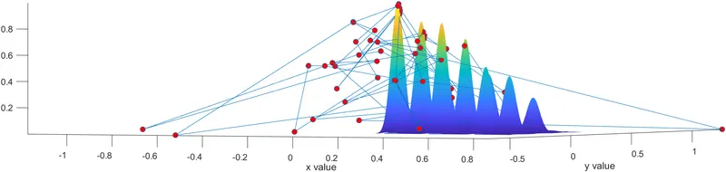
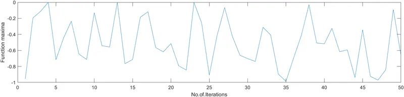
STUDY 1

-------------------------------------------------------------------------------------------------------------------

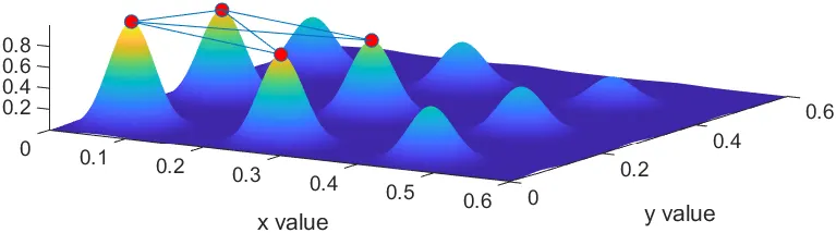
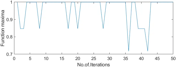
STUDY 2

-------------------------------------------------------------------------------------------------------------------

STUDY 3

-------------------------------------------------------------------------------------------------------------