Genetic Algorithm

Genetic Algorithm:

• A genetic algorithm (GA) is a method used to optimize various problems, which is actually based on Charles Darwin's evolution theory. It randomly repeats and changes the population of a particular problem. In its own context, it randomly picks up parents from a population, cross-links them to produce offspring of the next generation, and then repeats the process in the recent generation. Over multiple generations passed by, a perfect offspring will be established as an optimized product.
• GA is an inbuilt function in MatLab 'ga' and finds only the minimum of a function.
• So to find the maximum of a function using GA, the function needs to be made negative so that the ga will now inverse its output.
• Syntax of GA is created such that it's a function of the function we created: stalagmite, in this case, the number of variables used: 2 (x and y) in this case. It also depends on a function's equalities, inequalities, linearity, nonlinearity, limits(bounds), etc.

Stalagmite:

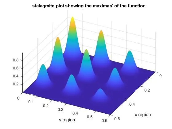
• Stalagmites are a group of sharp protruding objects that protrude from the ground or any source. A map that resembles the stalagmites is what it means in this context. Each sharp point is local maxima or local minima, depending on the problem. The highest point in the tallest peak is the global maximum or global minimum, depending on the problem.

Global maxima:

The function that is going to be optimized in this problem is

`f(x,y) = f_(1_x).f_(2_x).f_(1_y).f_(2_y)` where`

`f_(1_x) = [sin(5.1pix+0.5)]^6`; `f_(1_y) = [sin(5.1piy+0.5)]^6`

`f_(2_x) = exp[-4ln(2)(x-0.0667)^2/0.64]`; `f_(2_y) = exp[-4ln(2)(y-0.0667)^2/0.64]`

• A space is created: x and y ranging from 0 to 0.6 with 150 points in between using the linspace command.
• The x and y is created as a surface and meshed using the meshgrid command.
• A stalagmite plot is created for the above function by defining x and y length as the input variables
• Number of iterations for the studies is 100

Study 1:

• The GA for the above plot only gives two inputs and a function value of the global minimum. To get the global maximum, the function output should be negative. `f(x,y) = -( f_(1_x).f_(2_x).f_(1_y).f_(2_y))`
• It outputs results for variables x and y, but the GA function used random values as inputs. The random values can either be in the required plot region or scattered in space, or both.
• A for loop is created to find the input values through the GA function. It runs 100 iterations and deciphers 100 sets of input values.
• All the input values, along with the respective function maximum, are with the stalagmite surface.
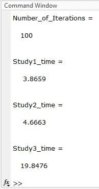
• The time taken to complete the process is calculated by the tic and toc function.

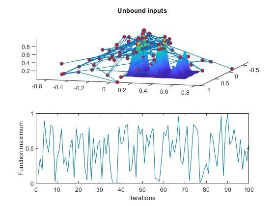
• Across 100 iterations, many fluctuations in the values can be seen, and visually, most of the inputs values found by the GA are scattered on and off the stalagmite plot in various places.
• It took 3.6 seconds to run 100 iterations for that function study.

Study 2

• Since the GA does not know which region to concentrate on to find the function maximums, along the old syntax of the GA, new additions such as upper limit and lower limits are added. Since there are no inequalities or equalities in the function, the blanks are denoted with [].
• An upper and lower limit of 0 to 1 is given for both the x and y regions.

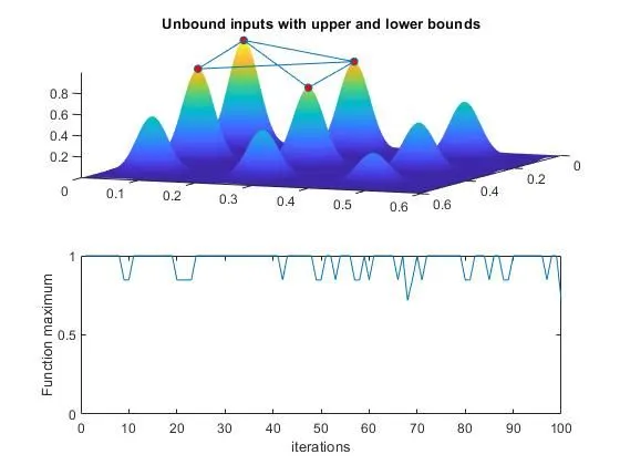
• It can be seen that the fluctuations in the iterations are zeroing out to a single value.
• Now the inputs derived only fall on the stalagmite plot because that is where the bounds are defined.
• It still didn't decipher on a single global maximum, but it displays four local maxima. This can be further shortened to a single point.
• It took 4.7 seconds to run this function study.

Study 3:

• To focus all the inputs only on the global maximum, the population is increased. The more the population, the more sampling can be done. More parent inputs will be crossed to optimize one final input set.
• The population is increased to 300 with the optionoptimize function in MatLab.
• The syntax for that inbuilt function is to have the ga set its population size.
• Then the ga syntax is added with the above options and then run to find the solution.

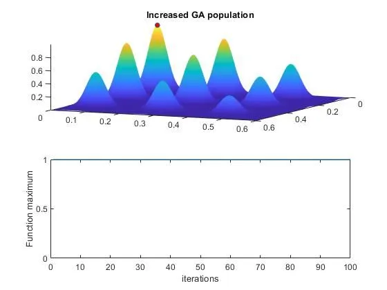
• Now, it all got reduced to one point where the actual global maximum is.
• This took 19.8 seconds to run the function study.
• The iterations are finalized to one value, and fluctuations can be noted.

The more the number of iteration or complexity of the function or population grows, the longer it takes to run the study

Codes:

clear all
close all
clc

%% defining the space
x = linspace(0,0.6,150);
y = linspace(0,0.6,150);
[x, y] = meshgrid(x,y); %meshing the space
f_max = get_stalagmite(x,y); %getting the inputs to create stalagmites
 
num_iters = 100; % to run the algorithm 100 times - number of iterations

%% Global Maxima
%to get the stalagmite surface which shows the global maxima
figure(1)
surfc(x,y,-f_max)
shading interp
title('stalagmite plot showing the maximas'' of the function')
xlabel('x region')
ylabel('y region')
 
% global maximum is found in the below portion
 %%  study 1 - statistical behavior
 tic
for i = 1:num_iters
     [input_max, fopt_max(i)] = ga(@stalagmite_max,2); %using GA to get optimized inputs
     xopt_max(i) = input_max(1);
     yopt_max(i) = input_max(2);
end
Study1_time = toc;

figure(2)
subplot(2,1,1)% creating subplots
hold on
surfc(x,y,-f_max)%creating stalagmite surface
shading interp%shading the stalagmite surface
plot3(xopt_max,yopt_max,-fopt_max,'marker','o','markersize',5,'markerfacecolor','r') %plotting GA outputs
title('Unbound inputs')
subplot(2,1,2)
plot(-fopt_max)
ylim([0 1]);
xlabel('iterations')
ylabel('Function maximum')

 %% study 2 - statistical behavior - with having upper and lower bounds
 tic
for i = 1:num_iters
     [input_max, fopt_max(i)] = ga(@stalagmite_max,2,[],[],[],[],[0;0],[0.6;0.6]);%using GA to get optimized inputs and setting upper and lower limits
     xopt_max(i) = input_max(1);
     yopt_max(i) = input_max(2);
end
Study2_time = toc;

figure(3)
subplot(2,1,1)
hold on
surfc(x,y,-f_max)
shading interp
plot3(xopt_max,yopt_max,-fopt_max,'marker','o','markersize',5,'markerfacecolor','r')
title('Unbound inputs with upper and lower bounds')
subplot(2,1,2)
plot(-fopt_max)
ylim([0 1]);
xlabel('iterations')
ylabel('Function maximum')

%% study 3 - Increasing the population
% {for 50 iterations and 2 variables x and y, the population will be 50
% sets of two random variable ie., 200

opt = optimoptions('ga');%adding options in GA syntax
opt = optimoptions(opt,'populationSize',300); %increasing the population size

tic
for i = 1:num_iters
     [input_max, fopt_max(i)] = ga(@stalagmite_max,2,[],[],[],[],[0;0],[0.6;0.6],[],[],opt); % increasing the GA population
     xopt_max(i) = input_max(1);
     yopt_max(i) = input_max(2);
end
Study3_time = toc;

figure(4)
subplot(2,1,1)
hold on
surfc(x,y,-f_max)
shading interp
plot3(xopt_max,yopt_max,-fopt_max,'marker','o','markersize',5,'markerfacecolor','r')
title('Increased GA population')
subplot(2,1,2)
plot(-fopt_max)
ylim([0 1]);
xlabel('iterations')
ylabel('Function maximum')

%time taken for each study for 100 iterations
Number_of_Iterations = num_iters 
Study1_time = Study1_time
Study2_time = Study2_time
Study3_time = Study3_time

%% Functions
function [fun] = get_stalagmite(x,y)
for i = 1:length(x)
     for j = 1:length(y)
         inp(1) = x(i,j);
         inp(2) = y(i,j);
         fun(i,j) = stalagmite_max(inp);
     end
 end
end
function [fun] = stalagmite_max(val)
A = val(1);
B = val(2);
f1A = (sin((5.1.*pi.*A)+0.5)).^6;
f2A = exp((-4.*log(2).*((A-0.0667).^2))./0.64);
f1B = (sin((5.1.*pi.*B)+0.5)).^6;
f2B = exp((-4.*log(2).*((B-0.0667).^2))./0.64);
fun =-(f1A.*f2A.*f1B.*f2B);
end