Week 4.1 - Genetic Algorithm
Genetic Algorithm (GA)
Genetic Algorithm (GA) is a search based optimization technique based on Darwin theory of Natural selection. It is mostly used to solve complex problems to determine the optimum solution, which otherwise would take lifetime to solve.
Optimization : Optimization refers to finding the values of input to determine the best possible output values. The best output can be determined by maximizing or minimizing the input functions.
Search space: Search space is the set of values which input will take. Here the process of optimization is to determine the point or value of input in the seach space which will give the best possible output.
Stalagmite Function : Stalagmite is a upward growing mound of mineral deposits that have precipated from water dripping onto the floor of a cave. Stalagmite function refers to a function with which we are generating values over a stalagmite kind of surface to determine local/global maxima and minimas.
To perform the optimization in Matlab we use in bullt GA function.
Natural Selection: There 5 steps in Genetic Algorithm :
1. Initial Population- Selecting the set of individuals to solve the problem called as population.
2. Fitness Function- Every solution is awarded a fitness score to evaluate how close the solution is to optimum desired solution.
3. Selection - Based on the fitness score the indiviaduals are selected and them genes to pass on to next generation.
4.Crossover - New individuals are generated by natural mutation. Offsprings are generated by exchanging the genes of parents among themselves untill crossover point is reached.
5.Mutation - For each offspring, select some genes and change its values.
Syntax:
x = ga(fun,nvars)x, to the objective function, fun. nvars is the dimension (number of design variables) of fun.
x = ga(fun,nvars,A,b,Aeq,beq,lb,ub)x, so that a solution is found in the range lb ≤ x ≤ ub. (Set Aeq=[] and beq=[] if no linear equalities exist.)
x = ga(fun,nvars,A,b,Aeq,beq,lb,ub,nonlcon,options)options. (Set nonlcon=[] if no nonlinear constraints exist.) Create options using optimoptions.
Matlab code to optimize the stalagmite function and determine the global maxima of function
clear all
close all
clc

%Defining our search space
x=linspace(0,0.6,150);
y=linspace(0,0.6,150);
num_spaces = 50;

% Creating 2D mesh
[xx yy] = meshgrid(x,y);
for i = 1:length(x)
    for j = 1:length(y)
        input_vector(1) = xx(i,j);
        input_vector(2) = yy(i,j);
        f(i,j) = stalagmite(input_vector);

    end
end

% Study 1 - Unbounded
 tic
 for i = 1:num_spaces
    [results,fopt(i)] = ga(@stalagmite,2);
    xopt(i) = results(1)
    yopt(i) = results(2)

 end
 study_time1 = toc

 figure(1)
 subplot(2,1,1)
 surfc(x,y,-f)
 shading interp
 hold on
 plot3(xopt,yopt,-fopt,'marker','o')
 subplot(2,1,2)
 plot(-fopt)
 xlabel('iterations')
 ylabel('function_maximum')

%study 2 - Bounded
tic
for i = 1:num_spaces
    [results,fopt(i)] = ga(@stalagmite,2,[],[],[],[],[0;0],[0.6;0.6]);
    xopt(i) = results(1)
    yopt(i) = results(2)
end
study_time2 = toc

figure(2)
subplot(2,1,1)
surf(x,y,-f)
shading interp
hold on
plot3(xopt,yopt,-fopt,'marker','o')
subplot(2,1,2)
plot(-fopt)
xlabel('iterations')
ylabel('function_maximum')

% study 3 - Increased Initial Population

options = optimoptions('ga')
options = optimoptions(options,'populationsize',250)
tic
for i = 1:num_spaces
    [results,fopt(i)] = ga(@stalagmite,2,[],[],[],[],[0;0],[0.6;0.6],[],[],options)
    xopt(i)= results(1)
    yopt(i)= results(2)
end

study_time3=toc
figure(3)
subplot(2,1,1)
surf(x,y,-f)
shading interp
hold on
plot3(xopt,yopt,-fopt,'marker','o')
subplot(2,1,2)
plot(-fopt)
xlabel('iterations')
ylabel('function_maximum')
Code for stalagmite fumction :
function A = stalagmite(input_vector)
x = input_vector(1);
y = input_vector(2);
f1 = (sin(5.1*pi*x+0.5)).^6;
f2 = exp((-4*log(2)*((x-0.0667).^2))/0.64);
f3 = (sin(5.1*pi*y+0.5)).^6;
f4 = exp((-4*log(2))*((y-0.0667).^2)/0.64);

A = -(f1*f2*f3*f4);

end
Code Explaination:
clear all
close all
clc
%Defining our search space
x=linspace(0,0.6,150);
y=linspace(0,0.6,150);
num_spaces = 50;
Using the above code 150 input values x and y are considered between 0 and 0.6 using linspace command.
The no.of iterations are taken as 50.
% Creating 2D mesh
[xx yy] = meshgrid(x,y);
for i = 1:length(x)
for j = 1:length(y)
input_vector(1) = xx(i,j);
input_vector(2) = yy(i,j);
f(i,j) = stalagmite(input_vector);
end
end
To plot 3D surface meshgrid is used to create 2D array of x and y and store them as input_vector
A Nested for loop is used to assign values from this array to input_vector.
This input vector is used as argument to call the stalagmite function later.
In the function code for stalagmite, output is taken -f since ga only minimizes the given function. But in our case we need the maximum value so we use -f as shown below.
function A = stalagmite(input_vector)
x = input_vector(1);
y = input_vector(2);
f1 = (sin(5.1*pi*x+0.5)).^6;
f2 = exp((-4*log(2)*((x-0.0667).^2))/0.64);
f3 = (sin(5.1*pi*y+0.5)).^6;
f4 = exp((-4*log(2))*((y-0.0667).^2)/0.64);
A = -(f1*f2*f3*f4);
end
Study 1 : Unbounded
tic
for i = 1:num_spaces
[results,fopt(i)] = ga(@stalagmite,2);
xopt(i) = results(1)
yopt(i) = results(2)
end
study_time1 = toc
figure(1)
subplot(2,1,1)
surfc(x,y,-f)
shading interp
hold on
plot3(xopt,yopt,-fopt,'marker','o')
subplot(2,1,2)
plot(-fopt)
xlabel('iterations')
ylabel('function_maximum')
Here inbulit ga is used to calculate the maxima of the function. Also ga is applied for random population for specified itierations.
The output is stored as results. The value at which maxima is obtained is stored as fopt.
In figure(1) subplot is used to get 2 plots insame figure.
In 1st subplot surf and plot3 are plotted.
surface is plotted for x,y,-f.
plot3 command is used to plot xopt,yopt and -fopt. Marker is used to mark the maximas.
In 2nd subplot, fopt is plotted to vsualise the optimum values at every iterations.
tic and toc is used to get the study time.
When the code is run we get below figure and output :
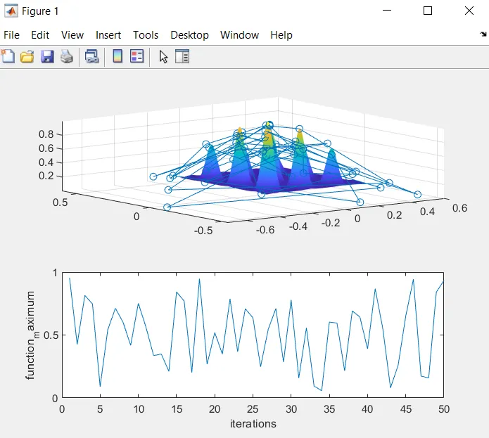
The optima values are outside the values of x and y hence failed to reach global maxime in 1st study.
Study time = 2.7731sec.
Study 2 : Bounded Values
tic
for i = 1:num_spaces
[results,fopt(i)] = ga(@stalagmite,2,[],[],[],[],[0;0],[0.6;0.6]);
xopt(i) = results(1)
yopt(i) = results(2)
end
study_time2 = toc
figure(2)
subplot(2,1,1)
surf(x,y,-f)
shading interp
hold on
plot3(xopt,yopt,-fopt,'marker','o')
subplot(2,1,2)
plot(-fopt)
xlabel('iterations')
ylabel('function_maximum')
lower and upper bounds of x and y are specified hence search is reduced with boundaries.
plotting is similar to above study.
The output is shown below :
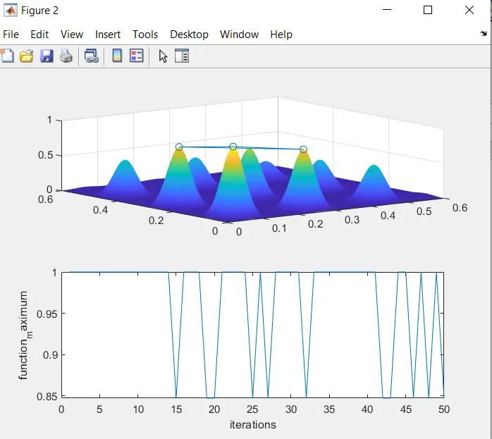
Though the optima values are within the limits it could not gave the exact maxima values.
Study time = 3.8sec
Study 3 - Increased initial population
options = optimoptions('ga')
options = optimoptions(options,'populationsize',250)
tic
for i = 1:num_spaces
[results,fopt(i)] = ga(@stalagmite,2,[],[],[],[],[0;0],[0.6;0.6],[],[],options)
xopt(i)= results(1)
yopt(i)= results(2)
end
study_time3=toc
figure(3)
subplot(2,1,1)
surf(x,y,-f)
shading interp
hold on
plot3(xopt,yopt,-fopt,'marker','o')
subplot(2,1,2)
plot(-fopt)
xlabel('iterations')
ylabel('function_maximum')
In this optimumoption is used and initial population is set to 250.
Plotting is similar to 1st study.
Output of this study is shown below :
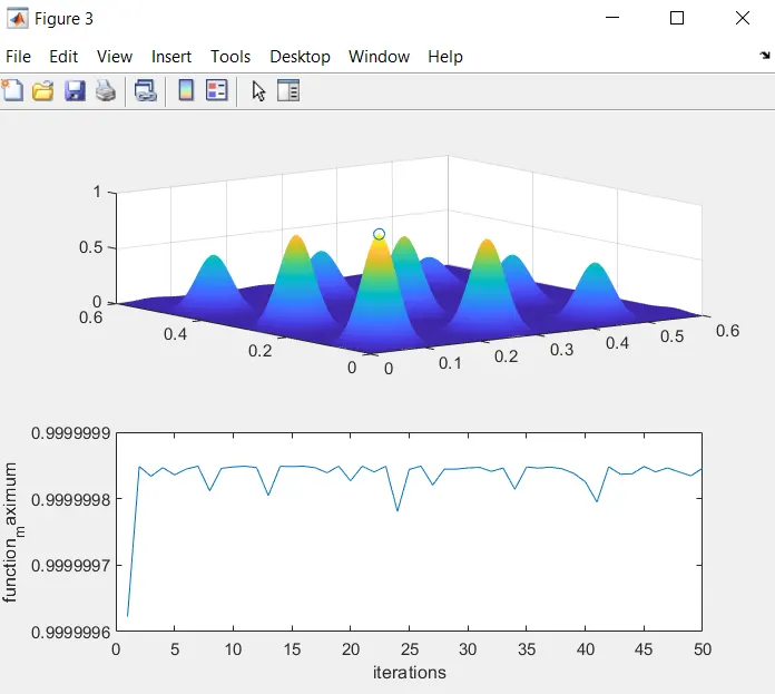
The right optimum value is determined in this study .
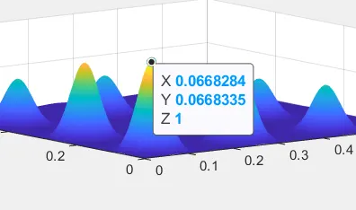
The study time is more compared to other studies i.e 11.93sec
All the output figures are attached.
Errors
1. Function code was not saved. Error1 attached
Solution : Function code saved again.
2. Syntax for bounded study was wrong. Error2 attached
Solution: parenthesis added.
3. Function was named as 'stagalmite'. But in main program 'stalagmite' was called (spell difference). error not attached.
Solution : Function name was corrected and called again.
References:
1.Matlab documentation for ga syntax.
2.https://in.mathworks.com/help/gads/options-in-genetic-algorithm.html