Week 3 - Solving second order ODEs

In Engineering, ODE is used to describe the transient behavior of a system. A simple example is a pendulum

The way the pendulum moves depends on the Newtons second law. When this law is written down, we get a second order Ordinary Differential Equation that describes the position of the "ball" w.r.t time.

Step 1 : ODE for pendulam

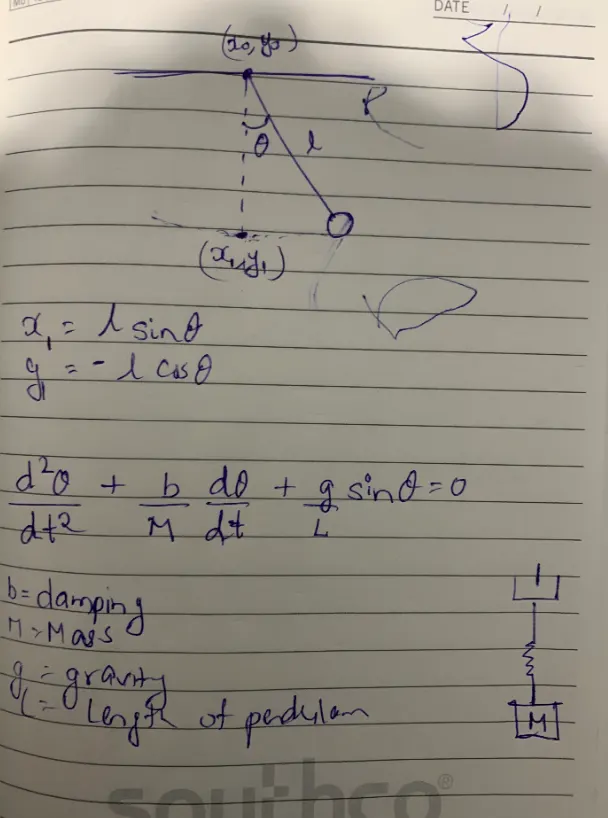
As shown above, damping of simple pendulam is represented by a second order ODE.

b=damping

m=mass in kg

g= gravity in m/sec^2

l=length of pendulam in m

The above eq is solved to determine theta and also rate at which theta changes wrt time. i.e velocity

The abover eq also dtermines motion of spring, mass and damper system

To solve this, 2nd order ODE is broken down to 1st order ODEs as shown below.

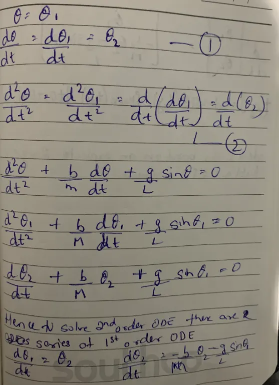
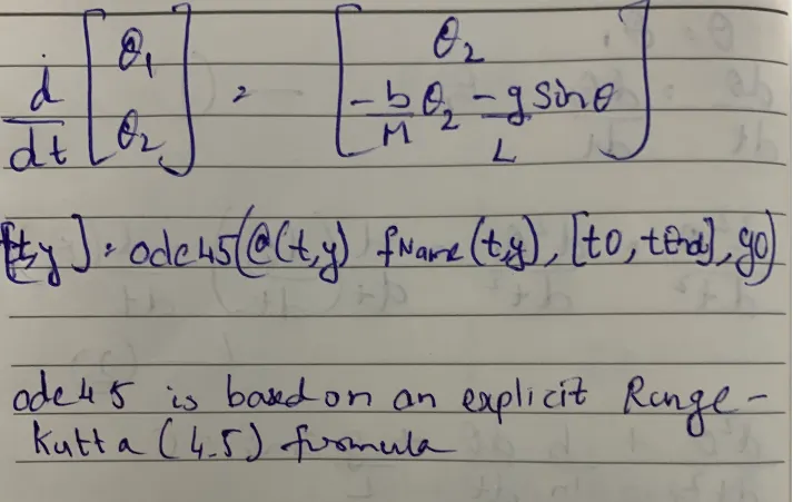
Step2: To solve the above ODE in matlab, ODE 45 function is used . The progam is shown below:

clear all
close all
clc

% inputs for the pendulum
b=0.05;
g=9.81;
l=1;
m=1;

% initial condition
theta_0 = [0,3];

% time points
t_span = linspace(0,20,500);

%  solve ODE
[t,results] = ode45(@(t,theta)ode_func(t,theta,b,g,l,m),t_span,theta_0);

%plotting
plot(t,results(:,1))
hold on
plot(t,results(:,2))
xlabel('Angular displament')
ylabel('Angular velocity')

% Animation to represent the motion of simple pendulam
x0 = 0;
y0 = 0;

ct=1;
for i = 1: length(t)
    x1 = l*sin(results(i,1));
    y1 = -l*cos(results(i,1));
    
    figure(2)
    plot([-1 1],[0 0],'linewidth',3,'color','b');
    axis([-2 2 -2 2]);
    line([x0 x1],[y0 y1],'linewidth',3,'color','g');
    hold on;
    plot(x0,y0,'O','markersize',3,'markerfacecolor','y');
    plot(x1,y1,'O','markersize',20,'markerfacecolor','r');
    title('Motion of Simple Pendulam')
    legend('Support rod','length of pendulam','fixed point','Ball of pendulam')
    grid on
    hold off
    M(ct)= getframe(gcf);
ct =ct+1;
end

%%videomaking
movie(M);
videofile = VideoWriter('Motion of Simple Pendulam.avi','uncompressed AVI');
open(videofile)
writeVideo(videofile,M)
close(videofile)

clear all close all clc to clear all prev commands

Inputs of the pendulam are defined as given in the assignment ie b,g,l and m.

The initial conditions are defined: theta_0 = [0,3]

Here 0 is anglur displacement and 3rad/s is angular velocity at time=0sec.

To inegrate tspan is defined between 0 to 20 sec and it has 500 values in between : t_span = linspace(0,20,500);

To solve ODE below syntax is used :

[t,results] = ode45(@(t,theta)ode_func(t,theta,b,g,l,m),t_span,theta_0);

Here t, results are the solution arrays. ode45 is a inbuilt solver in matlab which basically requires a dependant and independant variables. Here t is independent variable and theta is dependent variable.

ode_func(t,theta,b,g,l,m) : is the ode function defination which is wrtten as seperate program. this function has variables t,theta,b,g,l,m.

Integration limits are defined as tspan

and then initial conditions are defined as theta_0.

Step 3 : Before plotting lets see the ode function which is called here. Below is the program :

function [dtheta_dt] = ode_func(t,theta,b,g,l,m)

theta1 = theta(1);
theta2 = theta(2);
dtheta1_dt = theta2;
dtheta2_dt = -(b/m)*theta2 - (g/l)*sin(theta1);
dtheta_dt = [dtheta1_dt;dtheta2_dt];
end

Here theta 1 and theta2 are defined first.

Then we have the 2 ODEs which we solved earlier i.e dtheta1_dt and dtheta2_dt

both of these ode are combined into an array called as dtheta_dt (column matrix).

end is used to end the function.

This function code is attached as matlab program as ode_funct.

Step4 : Plotting the solution of ODE

Looking back at the main program, this subprogram when called will provide the output ie, time or t and results. results will be a column vector consisting of displacement and velocity at given time as we are solving 2 ODEs.

Figure1 : To plot the gragh of angular velocity and angular displacement.

plot(t,results(:,1))
hold on
plot(t,results(:,2))
xlabel('Angular displacment')
ylabel('Angular velocity')

plot is used to plot t and 1st column of results.

hold on to retain previous plot.

Next plot t and 2nd column results.

axis labels are defined.

This output is shown below:

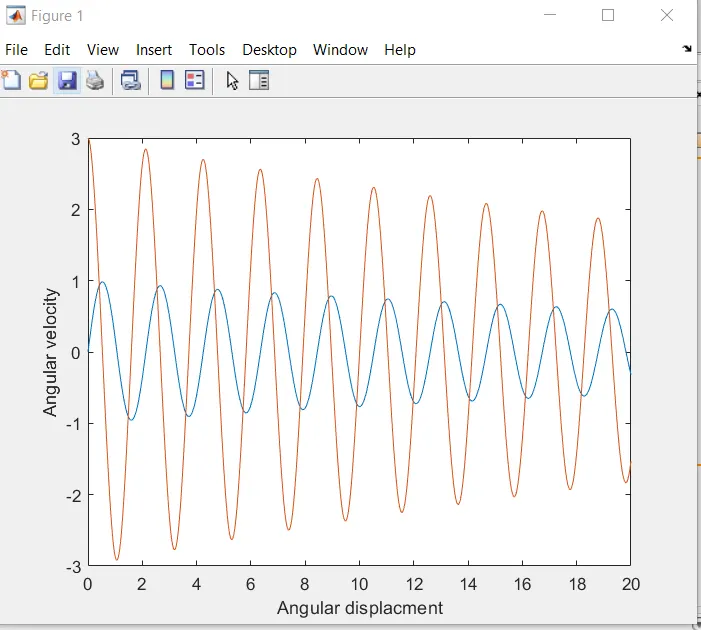
The output is also attached at 2nd ODE output.

Step5 : To animate the motion of pendulam below code is used.

x0 = 0;
y0 = 0;

ct=1;
for i = 1: length(t)
x1 = l*sin(results(i,1));
y1 = -l*cos(results(i,1));

x0 and y0 are set at (0,0)

counter is set at 1 , it actually represents each and every frame.

for loop is used repeat the set of instructions.

i is the array defined as length of time.

As shown in 1st image above x1 and y1 are defined. as the value of theta changes x1 will be at positive side and y1 will be negative side.

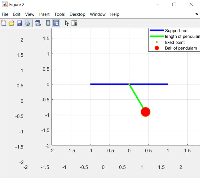
Figure 2 :

plot([-1 1],[0 0],'linewidth',3,'color','b');

in the above line support rod is plotted between -1 and 1 , linewidth is set to 3 and color is blue.

The axis values are set between -2 and 2.

line([x0 x1],[y0 y1],'linewidth',3,'color','g');

Here, Line command is used between x0, x1 and y0,y1.

hold on is used to retain the prev plot and line.

The below code is used to show the motion of ball :

plot(x0,y0,'O','markersize',3,'markerfacecolor','y');
plot(x1,y1,'O','markersize',20,'markerfacecolor','r');
title('Motion of Simple Pendulam')
legend('Support rod','length of pendulam','fixed point','Ball of pendulam')
grid on
hold off

x0, yo is plotted as fixed point.

x1,y1 is plotted with marker 'O' and size 20 and colour red.

The title of figure is given as 'Motion of Simple Pendulam'.

The legends are defined in order.

grid is turned on.

To get the figues of each iteration getframe is used.

counter is incremented for next values.

end is put to complete the loop.

The output is shown below:

Step6 : To make the video file below code is used:

movie(M);
videofile = VideoWriter('Motion of Simple Pendulam.avi','uncompressed AVI');
open(videofile)
writeVideo(videofile,M)
close(videofile)

movie(M) is a matrx which captures all the frames.(getframe(gcf) is used prev )

VideoWriter is the command to create a video in .avi format with name of video file

open(videofile) - this will open the video once after plotting.

writeVideo - this will save the video in it.

close(videofile) - this will close the file

Hence a video file will be saved where the program is saved.

The final matlab code files are attached as ode_pendulum_challenge.

The video as output is uploaded in Youtube. the link is : https://youtu.be/LHA1js8ntNI

The picture of animation plot is also attached as pendulam animation output.

Errors occured before executing the programn are shown. All the error screenshots are also attached with same errot numbers

1. error 1 :

Mistake : invalid ode45 command.

Solution: @ is added before the variables.

2.error 2 :

Mistake : sind was used. hence the plots were incorrect

Solution: changed to sin. The inputs are in radians not degrees.

3.error 3 :

Mistake : colon was used instead of semicolon. dtheta_dt has to be column matrix.

Solution: semicolon was used to get column matrix.

4.error 4 :

Mistake : pendulam plotted upwards

Solution: -ve used to define y1.

5.error 5 :

Mistake : Pendulam motion was showing trails of the images

Solution: Hold off added to plot the current motion of theta value in pendulam.

6.error 6:

Mistake - videowriter was typed

Solution- case changed to videofile = VideoWriter