Week 4.1 - Genetic Algorithm

%coding stalagmite function

function[f] = stalagmite(inputvector)

a = inputvector(1);
b = inputvector(2);

f1x = (sin((5.1*pi*a) +0.5))^6;
f1y = (sin((5.1*pi*b) +0.5))^6;

f2x = exp(-4*log(2)*(((a-0.0667)^2)/0.64));
f2y = exp(-4*log(2)*(((b-0.0667)^2)/0.64));

[f] = -(f1x*f1y*f2x*f2y);

end

%genetic algorithm, optimisation
clear all
close all
clc

%defining search space
x = linspace(0,0.6,150);
y = linspace(0,0.6,150);

%creating 2D mesh
[xx, yy] = meshgrid(x,y);

%no. of iterations for study: 50
num_case = 50;

%evaluating the stalagmite function

for i=1:length(xx)
    for j = 1:length(yy)
        inputvector(1)=xx(i,j);
        inputvector(2)=yy(i,j);
        f(i,j) = stalagmite(inputvector);
    end
end

%generating surface plot
figure(1)
surfc(xx,yy,-f)

shading interp

%Unbound statistical behaviour

tic

for a=1:num_case
    
    [inputs,fop(a)] = ga(@stalagmite,2);
    xop(a) = inputs(1);
    yop(a) = inputs(2);
    
end

study1_time = toc

%graph plot

figure(2)

subplot(2,1,1)

surfc(xx,yy,-f)
hold on
shading interp
plot3(xop,yop,-fop,'marker','o','markersize',3)
xlabel('x')
ylabel('y')

subplot(2,1,2)

plot(fop)
xlabel('iterations')
ylabel('function value')


%Bound statistical behavior

tic

for b = 1:num_case
   
    [inputs,fop(b)] = ga(@stalagmite,2,[],[],[],[],[0;0],[1;1]);
    xop(b)= inputs(1);
    yop(b)= inputs(2);
end

study2_time = toc

%graph plot

figure(3)

subplot(2,1,1)

surfc(xx,yy,-f)
hold on
shading interp
plot3(xop,yop,-fop,'marker','o','markersize',3)
xlabel('x')
ylabel('y')

subplot(2,1,2)

plot(fop)
xlabel('iterations')
ylabel('function value')


%study3
options = optimoptions('ga');
options = optimoptions(options,'PopulationSize',400)

tic

for c = 1:num_case
   
    [inputs,fop(c)] = ga(@stalagmite,2,[],[],[],[],[0;0],[1;1],[],[],options);
    xop(c)= inputs(1);
    yop(c)= inputs(2);
end

study3_time = toc

%graph plot

figure(4)

subplot(2,1,1)

surfc(xx,yy,-f)
hold on
shading interp
plot3(xop,yop,-fop,'marker','o','markersize',3)
xlabel('x')
ylabel('y')

subplot(2,1,2)

plot(fop)
xlabel('iterations')
ylabel('function value')

Outputs:

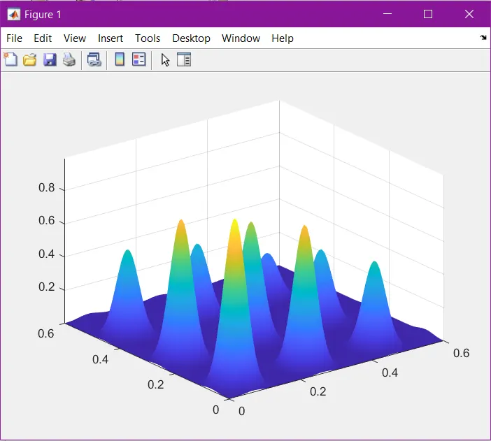
Study1:

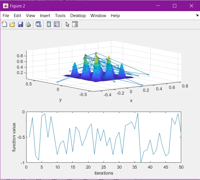
Study2:

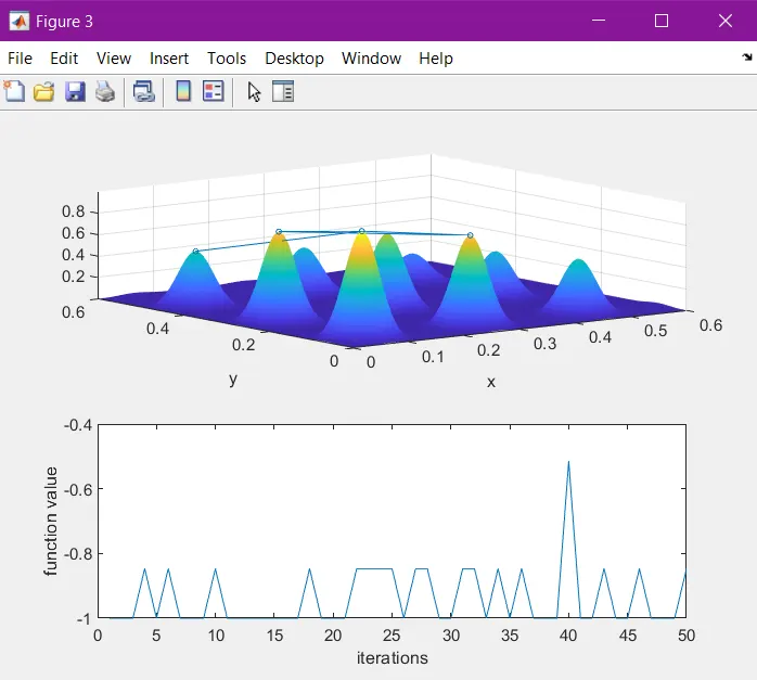
Study3:

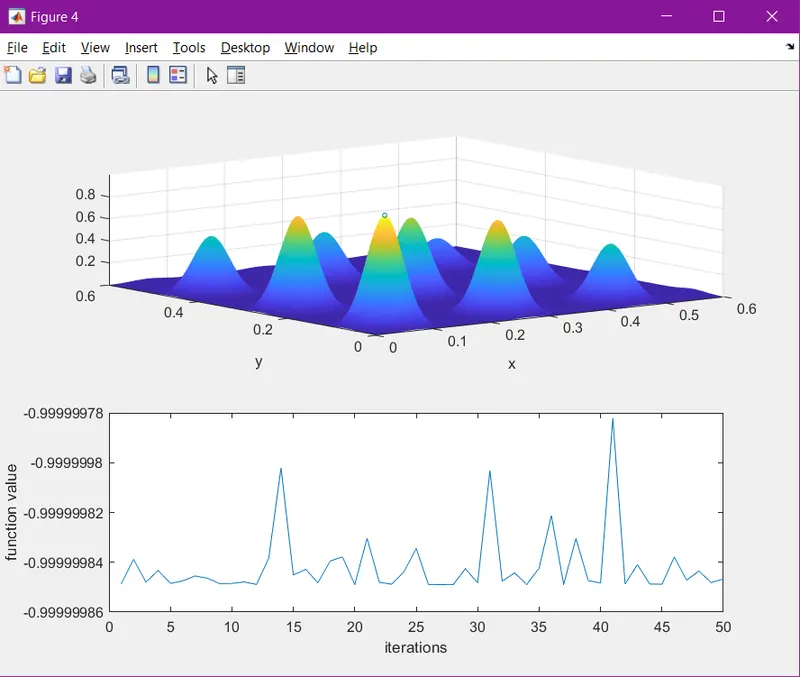
Genetic Algorithm:

This algorithm is used to find the optimum solution for a set of data. The genetic algorithm selects the best (fittest) optimum data from the original set (1st generation) and the second set of data (2nd generation) is created by the crossover of the initially selected values. The selection of the data depends on the fitness function. The created data points (offsprings) may have the more or less fittness value when compared to their parents. The created values (second generation) goes under the same process as before untill the algorithm finds out that the crossover and mutation is leading to the same values in the next generation. At this point, the algorithm will terminate. Thus, the process continues untill the highest possible 'best' value is obtained. This is called the global optima.

Syntax of ga: In the code the ga syntax is as follows

[x,fval] = ga(fun,nvars)

where x = 'input' in our code.

fval = 'fop', which is the fitness function values

fun = '@stalagmite', the fitness function which was defined

nvars = '2', the number of variables

Code explaination:

The stalagmite function was coded as per the given equations. The 'ga' finds the 'minima' in MATLAB, hence the negative output was defined for the function. The searchspace was defined for the initial set of points (first generation).A meshgrid was created using the search space values. For loop was used to input the meshgrid values in the stalagmite function. Them the stalagmite function was visualised using the 'surfc' command and 'shading interp' command was used to neglect the surface lines. 'num_case' was defined, which indicated the number of iterations performed by ga.

Study1:

The 'ga' syntax was used to get the values of 'fop' and the 'xop' and 'yop' were fed the 'input' values. 'tic-toc' command was used to display the time taken for the iteration. Here the ga is given freedom to take values from any range. Thus, the output will vary everytime the code is run. The output is plot using the 'plot3' command to visualise the values in 3-D.

Study2:

This time the 'ga' is bound to take values between an upper limit and lower limit defined in the syntax. This reduces the variation in the optimum value and thus accuracy towards the global optima increases

Study3:

The 'optimoptions' command was used to increase trhe size population within the bound conditions. This increases the probability of finding better and most viable global optima. Thus the accuracy towards the global optima is highest in this study. However, the large population will increase the code running time.