Week 4.1 - Genetic Algorithm

Aim: Write a code in MATLAB to optimize the stalagmite function and find the global maxima of the function.

Objective:

• Write a code in MATLAB to optimizethe stalagmite function and find the global maxima of the function.
• Plot graphs for all 3 studies and for F maximum vs no. of iterations.

Theory:

Optimization: Optimization is the process of making something better. In any process, we have a set of inputs and a set of outputs as shown in the following figure.

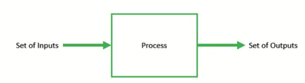
Optimization refers to finding the values of inputs in such a way that we get the “Best” output values. The definition of “Best” varies from problem to problem, but in mathematical terms, it refers to the maximizing or minimizing one or more objective functions, by varying the input parameters.

GA (Genetic Algorithm):

Nature has always been a great source of inspiration to all manking. Genetic Algorithm (GAs) aresearch based algorithms based on the concepts of “Charles Darwin’s” Natural selection & genetics. These are intelligent exploitation of random search provided with historical data to direct the search into region of better proformance in solution space. They are commonly used to generate high-quality solutions for optimization problems and search problems.

The algorithm is based on the survival of the fittest concept.

There are Five phases in Genetic Algorithm

1. Initial Population
2. Fitness Function
3. Selection
4. Crossover
5. Mutation

This principle of Genetic algorithm is also adopted in Statistics, programs, artificial intelligence, to solve optimization problems. Etc.

The Genetic Algorithm is a method for solving both constrained and unconstrained optimization problems that is based on natural selection, the process that drives biological evolution. The genetic algorithm repeatedly modifies a population of individual solutions. At each step, the genetic algorithm selects individuals at random from the current population to be parents and uses them to produce children for the next generation. Over successive generations, the populations “evolves” towards an optimal solution.

The genetic algorithm uses three main types of rules at each step to create the next generation from the current population.

• Selection rules select the individuals, called parents, that contributes to the population at the next generation.
• Crossover rulescombine two parents to form children for the next generation.
• Mutation rulesapply random changes in individual parents to form children.

Syntax

x = ga(fun,nvars)

x = ga(fun,nvars,A,b)

x = ga(fun,nvars,A,b,Aeq,beq)

x = ga(fun,nvars,A,b,Aeq,beq,lb,ub)

x = ga(fun,nvars,A,b,Aeq,beq,lb,ub,nonlcon)

x = ga(fun,nvars,A,b,Aeq,beq,lb,ub,nonlcon,options)

x = ga(fun,nvars,A,b,[],[],lb,ub,nonlcon,IntCon)

x = ga(fun,nvars,A,b,[],[],lb,ub,nonlcon,IntCon,options)

x = ga(problem)

[x,fval] = ga(___)

[x,fval,exitflag,output] = ga(___)

[x,fval,exitflag,output,population,scores] = ga(___)

Formula

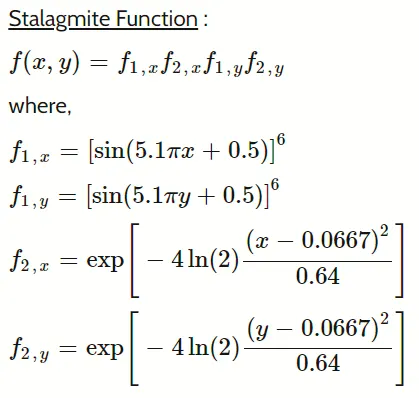
Function program:

function[F] = stalagmite_func(input_vector)
  
  x = input_vector(1);
  y = input_vector(2);
  
  f1_x = (sin(5.1*pi*x+0.5)).^6;
  f1_y = (sin(5.1*pi*y+0.5)).^6;
  
  f2_x = exp(-4*log(2)*((x-0.0667).^2)/0.64);
  f2_y = exp(-4*log(2)*((y-0.0667).^2)/0.64);
  
  [F] = -(f1_x.*f1_y.*f2_x.*f2_y);
  end

Main program:

clear all
close all
clc

% Defining search space

% One Dimensional
x = linspace(0,0.6,150);
y = linspace(0,0.6,150);

% Creating a 2D Mesh
[xx yy] = meshgrid(x,y);


% Evaluating Stalagmite function
for i = 1:length(xx)
      for j = 1:length(yy)
      input_vector(1) = xx(i,j);
      input_vector(2) = yy(i,j); 
      f(i,j) = stalagmite_func(input_vector);
   endfor

endfor

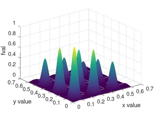
figure(1)
surfc(xx,yy,-f)
xlabel('x value')
ylabel('y value')
zlabel('fval')
shading interp
[inputs,fval] = ga(@stalagmite_func,2);


%% Study 1: Unbounded statistical Behaviour
tic
num_cases = 50;
for i = 1:num_cases
    [inputs, fopt(i)] = ga(@stalagmite_func,2);
    xopt(i) = inputs(1);
    yopt(i) = inputs(2);
 endfor
study1_time = toc
F=-f;

% Study 1 Plotting
figure(2)
subplot(2,1,1)
hold on
surfc(x,y,F)
shading interp
plot3(xopt,yopt,-fopt,'marker','o','markersize',5,'markerfacecolor','r')
title('Unbounded Inputs')
xlabel('x')
ylabel('y')
zlabel('F')
subplot(2,1,2)
plot(-fopt)
xlabel('Iterations')
ylabel('Function maximum')



%% Study 2: Statistical Behaviour with lower & upper bounds
tic
num_cases = 50;
for i = 1:num_cases
  [inputs,fopt(i)] = ga(@stalagmite_func,2,[],[],[],[],[0;0],[0.6;0.6]);
  xopt(i) = inputs(1);
  yopt(i) = inputs(2);
    
  endfor
study2_time = toc
F=-f;

% Study 2  Plotting

figure(3)
subplot(2,1,1)
hold on
surfc(x,y,F)
shading interp
plot3(xopt,yopt,-fopt,'marker','o','markersize',5,'markerfacecolor','r')
title('Bounded Inputs')
xlabel('x')
ylabel('y')
zlabel('F')
subplot(2,1,2)
plot(-fopt)
xlabel('Iterations')
ylabel('Function maximum')


%% Study 3: Increasing GA iterations

options = gaoptimset('PopulationSize',300);
tic
num_cases = 50;
for i = 1:num_cases
  [inputs,fopt(i)] = ga(@stalagmite_func,2,[],[],[],[],[0;0],[0.6;0.6],[],options);
  xopt(i) = inputs(1);
  yopt(i) = inputs(2);
    
  endfor

study3_time = toc
F=-f;

% Study 3  Plotting

figure(4)
subplot(2,1,1)
hold on
surfc(x,y,F)
shading interp
plot3(xopt,yopt,-fopt,'marker','o','markersize',5,'markerfacecolor','r')
title('Bounded Inputs with modified population size')
xlabel('x')
ylabel('y')
zlabel('F')
subplot(2,1,2)
plot(-fopt)
axis([0 50 0 1.5])
xlabel('Iterations')
ylabel('Function maximum')
FMAX = -min(fopt);
X = mean(xopt);
Y = mean(yopt);

Program Steps:

Step 1: Clearing workspace, command window and closing all plots

Step 2: Define our search space by using linspace command

Step 3: Calculating 2Dinsional mesh using meshgrid command

Step 4: Evaluating Stalagmite function for each value of x & y

Note - In Command window load ga & optim packages, (optim is not yet released as of now).

pkg load ga

Step 5: Study_1 - GA command with unbounded inputs. For unbounded GA, the optimum value may be obtained from outside of search space.

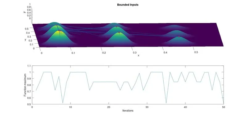
Step 6: Study_2 - GA command with bounded inputs. The optimum value will be obtained from outside of search space since the search is bounded within the population. However there will be a huge variation in optimum value.

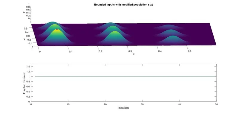
Step 7: Study_3 - GAoptimset command with bounded inputs would give an optimum value from within the search space and also to be noted that the population size is increased to 300 which will further refine the optimal value.

Note - gaoptimset command is used instead of optimoptions

Results & discussions:

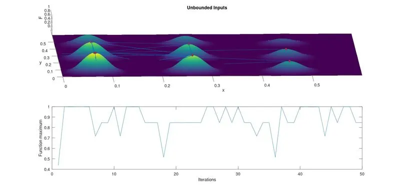
Study 1 | UnBounded input population

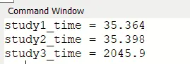
Time taken to perform the evaluation - 35.364 seconds

The Optimum values lies between 0.5 to 1 (Unconstrained Minima value)

Study 2 | Bounded input population

Time taken to perform the evaluation - 35.398 seconds

The Optimum values lies between 0.5 to 1 (But most vlaues lies at 1, showing that the boundary is more narrowed and within limit)

Study 3 | Bounded input population optimized

Time taken to perform the evaluation - 2045.9 seconds (due to the gaoptimset command)

The Optimum values lies at 1

Based on the research the answer for the following are:

Stopping Criteria-

When there has been no improvement in the population for X iterations

• When we reach an absolute number of generations.
• When the objective function value has reached a certain pre-defined value.

Significance of running multiple iterations-

• Multiple iterations are doen to get the Global Maxima in the desied range. The main objective is to get only 1 desired optimum value for the givewn problem.