Week 4.1 - Genetic Algorithm

Objective : Write a code for genetic algorithm to optimise the stalagmite function.

Aim : Code in MATLAB should optimise the stalagmite function and would determine the global maxima of the function.

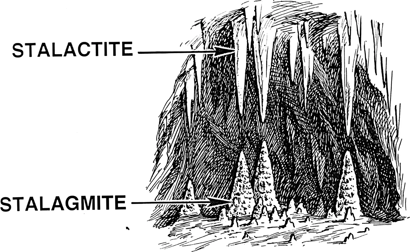
Theory : There are two basic shapes that are introduced with the terms stalagmite and stalactites. Stalactites and the Stalagmites are natural formtion happening in the caves due to mineral deposits. Stalactites are the types that are stuck to the ceiling that hang down pointing towards the floor; Stalagmites are almost similar to Stalactites but are facing towards the ceiling. These shapes also have their importance in the mathematical field as shapes that represent this type of formation.                                                           

                                                                  

Genetic Algorithms :

Optimization of a Non-Linear problem is done by this GENETIC ALGORITHM technique. It is based on the darwin's theory of evolution or also commmonly known as survival of the fittest and assists in finding the global minima of the optimization problem. The objective function is being tested against an initial test of solutions. The process helps the successive generations to be evolved done in 5 phases

1) Initial Population

The process begins with initialization, whereby an initial population of candidate solutions is generated. There are many various ways of initializing populations, however, with Genetic Algorithms, the foremost fashionable methodology of initialization is solely to make a population of random initialized binary strings. Once the initial population has been created, the biological process people cycle begins.

2) Selection

At each generational step, a pool of parents is chosen from the parent population based on the fitness values of each individual using a selection mechanism, such that the fittest individuals will have a greater probability of passing on genetic material to subsequent generations. This selected population (known as the “parent” population) then forms the basis for all subsequent optimizations during the generational step.

3) Variation

Once the parent population is fully populated via the selection process, a child population is created which will form the basis of the next generation. This child population is generated by variation operators, which are performed on individuals from the parent population. The most prominent such methods are crossover and mutation.

4) Cross-over

Crossover takes pairs of parents from the parent population (usually random selection with replacement, such that the same parent can be selected multiple times to produce children). These parents then have some of their genetic information swapped between them. Crossover is typically performed on randomly selected pairs of parents from the parent population until the new “child” population reaches the same size as the original parent population.

5) Mutation

While crossover simply swaps pre-existing information between pairs of candidate solutions, mutation in Evolutionary Algorithms is typically the standard method of introducing “new” genetic material into the population. Once the child population has been created via crossover, mutation in canonical Genetic Algorithms then occurs on all children in a “bit-flip” fashion by randomly changing codons on the chromosome between 0 and 1

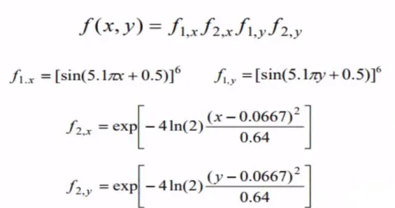
FORMULAS

EXPLAINATION

A random array was generated of the "x" & "y" values; mesh grid was used to creat a 2d array of the same. A nested loop was used to assign the values from the current array to the stalagmite function array namely (in_vec). This function is written seperately and is given at the bottom. GA in general is used to find the global minima hence a minus sign is used in the output of function to get the global maxima. For getting the time take the tic-toc command is used for ever case. CASE 1 uses no bounds for creating the plots; the "-" sign is given to the f as to get the stalagmite upwards. CASE 2 bounding is introduced so as to get more accurate results. Then in CASE 3 number of population is increased to get even more accurate with the result whilst the more the population the slower the  GA runs. Then Case 3 gives us the desired values of the global maxima.

Stopping criteria:

1) The algorithm stops when number and value of generations becomes the same

2) The algorithm stops when the value of fitness function for the best point in the current population is less than or equal to the fitness limit. 

CODE

close all
clear all
clc

x = linspace(0,0.6,150);
y = linspace(0,0.6,150);
num_cases = 40;

%2D array
[xx yy] = meshgrid(x, y);

for i= 1:length(xx)
    for j = 1:length(yy)
        in_vec(1) = xx(i,j);
        in_vec(2) = yy(i,j);
        f(i,j) = stalagmite_func(in_vec);
    end
end

tic
for i = 1:num_cases
    [input,fopt(i)] = ga(@stalagmite_func, 2);
    xopt(i) = input(1);
    yopt(i) = input(2);
end
case_time_1 = toc
    
figure(1)
subplot(2,1,1)
hold on
surfc(xx,yy,-f)
xlabel('x')
ylabel('y')
title('Case 1','color','k')
shading interp
plot3(xopt,yopt,-fopt,'marker','o','markersize',5,'markerfacecolor','r');
subplot(2,1,2)
plot(-fopt)
xlabel('Iterations')
ylabel('Function maximum')


%case 2

tic
for i = 1:num_cases
    [input,fopt(i)] = ga(@stalagmite_func, 2,[],[],[],[],[0;0],[0.5;0.5]);
    xopt(i) = input(1);
    yopt(i) = input(2);
end
case_time_2 = toc
    
figure(2)
subplot(2,1,1)
hold on
surfc(xx,yy,-f)
xlabel('x')
ylabel('y')
title('Case 2','color','k')
shading interp
plot3(xopt,yopt,-fopt,'marker','o','markersize',5,'markerfacecolor','r');
subplot(2,1,2)
plot(-fopt)
xlabel('Iterations')
ylabel('Function maximum')

%case 3
options = optimoptions('ga');
options = optimoptions(options,'PopulationSize',170);


tic
for i = 1:num_cases
    [input,fopt(i)] = ga(@stalagmite_func, 2,[],[],[],[],[0;0],[0.5;0.5],[],[],options);
    xopt(i) = input(1);
    yopt(i) = input(2);
end
case_time_3 = toc
    
figure(3)
subplot(2,1,1)
hold on
surfc(xx,yy,-f)
xlabel('x')
ylabel('y')
title('Case 3','color','k')
shading interp
plot3(xopt,yopt,-fopt,'marker','o','markersize',5,'markerfacecolor','r');
subplot(2,1,2)
plot(-fopt)
xlabel('Iterations')
ylabel('Function maximum')

display(input)

Function

function f = stalagmite_func(in_vec)
f1x = (sin((5.1*pi).*in_vec(1)+0.5)).^6;
f1y = (sin((5.1*pi).*in_vec(2)+0.5)).^6;

f2x = exp((((in_vec(1)-0.0667).^2)/0.64).*(-4*log(2)));
f2y = exp((((in_vec(2)-0.0667).^2)/0.64).*(-4*log(2)));
f1 = f1x*f1y*f2x*f2y;
f = -f1;
end

Input values

x = 0.0668

y = 0.0668