Week 4.1 - Genetic Algorithm
Aim:
Write a code in MATLAB to optimise the stalagmite function and find the global maxima of the function.
Objective:
- Clearly expalin the concept of genetic algorithm in your own words and also explain the syntax for ga in MATLAB in your report.
- Make sure that your code gives the same output, even if it is made to run several times.
- Plot graphs for all 3 studies and for F maximum vs no. of iterations. Title and axes labels are a must, legends could be shown if necessary.
Theory:
Optimisation is a decision making process,it helps to find the best results under a set of prioritized criteria and constraints,which is executed iteratively by comparing various solution till a optimum or satisfactory solution is found.
The following procedure followed by optimisation process,
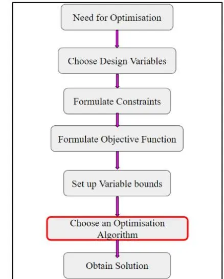
As we know the above in the flow chart,we need to choose a optimisation algorithm to perform the optimisation process.Genetic algorithm is a optimisation process.
Genetic Algorithm (GA) is a search based optimisation technique based on the principle of genetic and natural selection.It is frequently used to solve the optimisation problems,in research and machine learning.
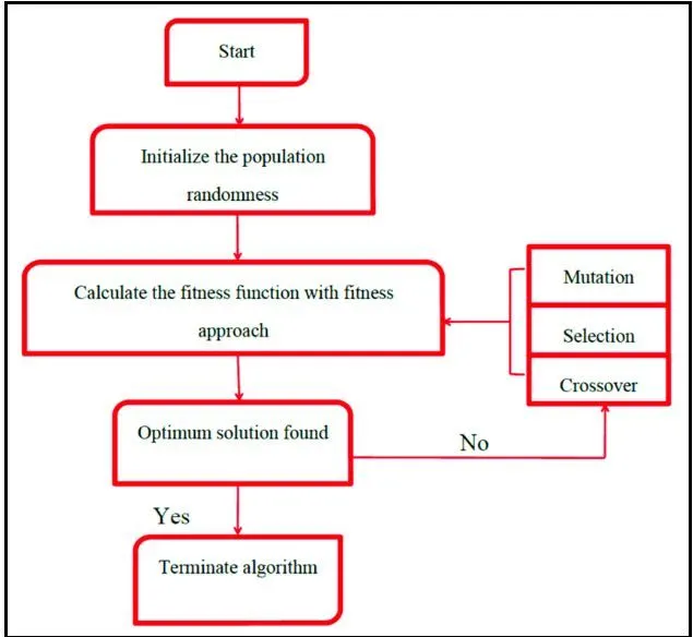
Genetic Algorithm optimisation starts with initialization,
Population is the number of sample data points taken to perform the genetic algorithm operation.
Sample data points goes through following three steps,
- Selection
- cross over
- Mutation
Selection
In this step parents are taken as the sample data points,the main procedure of selection process is to select higly fit individuals.
Cross-Over
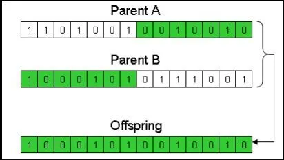
It is the process of taking two parent's solutions and producing the child for them,There are many way to solve the cross over process.
The following method is known as a one-point crossover method, where the set of genes from Parent A is combined with Parent B to create a new offspring.
Here 0 and 1 represents the genes,
Mutation
Mutation is carried out to maintain the genetic diversity from one generation of a population of chromosomes to the next.
If mutation is not performed, the chromosomes will become too similar to each other, convergence takes place soon and results in local minima.
Similar to the crossover, there are many ways to perform the mutation process.
example:Swap Mutation.
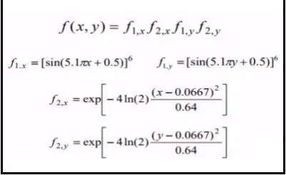
Genetic Algorithm optimisation for a stalagmite function, to find its minima. The stalagmite function is,
Code For Finding The Global Maxima Of The Stalagmite Function
 clear all
close all
clc

 %Defining our search space
 x = linspace(0,0.6,150);
 y = linspace(0,0.6,150);
 num_cases =50

 %Creating a 2Dimensional mesh
 [xx,yy] = meshgrid(x,y);

 %Evaluating the stalagmite function

 for i=1:length(xx)
     for j =1:length(yy)
         input_vector(1) = xx(i,j);
         input_vector(2) = yy(i,j);

         f(i,j)= stalagmite(input_vector);

     end

 end

 %Study_1 Unbound
 tic
    for  r=1:num_cases
  [input,fopt1(r)]=ga(@stalagmite,2);
  xopt1(r)=input(1);
  yopt1(r)=input(2);

  end


 study1=toc

 %plotting the data
 figure(1)
 subplot(2,1,1)
  hold on
 surfc(x,y,-f)
 shading interp
 xlabel('x axis')
 ylabel('y axis')
 zlabel('z axis')

 plot3(xopt1,yopt1,-fopt1,'marker','o','markerfacecolor','r','markersize',5)
 title('Study 1')
 subplot(2,1,2)
 plot(-fopt1)
 xlabel('Iteration')
 ylabel('Function maxima')


 %study_2 Statistical behaviour with upper bound and lower bound
  tic
 for r=1:num_cases
     [input,fopt2(r)]=ga(@stalagmite,2,[],[],[],[],[0,0],[0.6,0.6]);
     xopt2(r)=input(1);
     yopt2(r)=input(2);
 end
study2=toc

  %plotting the data
 figure(2)
 subplot(2,1,1)
  hold on
 surfc(x,y,-f)
 shading interp
 xlabel('x axis')
 ylabel('y axis')
 zlabel('z axis')

  plot3(xopt2,yopt2,-fopt2,'marker','o','markerfacecolor','r','markersize',5)
 title('Study 2')
 subplot(2,1,2)
 plot(-fopt2)
 xlabel('Iteration')
 ylabel('Function maxima')

 %study3 GA Increasing Iteration
 options=optimoptions('ga');
 options=optimoptions(options,'populationsize',200);

 tic
 for r=1:num_cases
     [input,fopt3(r)]=ga(@stalagmite,2,[],[],[],[],[0,0],[0.6,0.6],[],[],options);
     xopt3(r)=input(1);
     yopt3(r)=input(2);

 end
 study3=toc

 %plotting the data
 figure(3)
 subplot(2,1,1)
 hold on
 surf(x,y,-f)
 shading interp
 xlabel('x-axis')
 ylabel('y-axis')
 zlabel('Z-axis')


 plot3(xopt3,yopt3,-fopt3,'marker','o','markerfacecolor','r','markersize',5)
 title('Study 3')
 subplot(2,1,2)
  plot(-fopt3)
 xlabel('Iteration')
 ylabel('Function maxima')
Step Wise Explanation To The Code:
 clear all
close all
clc

 %Defining our search space
 x = linspace(0,0.6,150);
 y = linspace(0,0.6,150);
 num_cases =50

 %Creating a 2Dimensional mesh
 [xx,yy] = meshgrid(x,y);
Program starts with clear all close all and clc to clear and close the file opened in the command window,In search space we are creating a 1 dimensional array X and Y, for X and Y is defined in the range of 0 to 0.6. So in this 150 values will be taken for the evaluation.
num_cases is to run ga for the function in the loop. So all the x and y values are saved in the meshgrid command which is stored in xx and yy.
 %Evaluating the stalagmite function

 for i=1:length(xx)
     for j =1:length(yy)
         input_vector(1) = xx(i,j);
         input_vector(2) = yy(i,j);

         f(i,j)= stalagmite(input_vector);

     end

 end
In this command for each value of X and Y we are creating an array called input_vector, so this input vector is a row vector, meaning it has two coloumns. we have x value and y value so take the 2nd value and put them in an array that is input vector .
There is a function called Stalagmite so this function takes the input vector and calculate f. the values are calculated from the function.And from input vector x and y calculate the position which is stored in i and j, with this position function will setup the value of the function at each position.
In both xx and yy there will be 150x150 matrics.
 %Study_1 Unbound

 tic
    for  r=1:num_cases
  [input,fopt1(r)]=ga(@stalagmite,2);
  xopt1(r)=input(1);
  yopt1(r)=input(2);

  end


 study1=toc
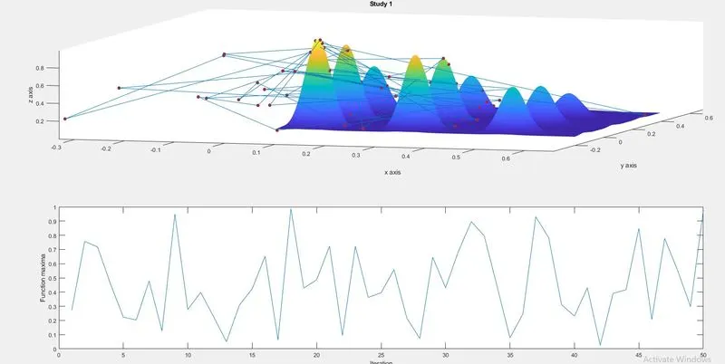
In this command random values will be calculated from the function and we get results for study 1, So here ga function is used to run stalagmite data and give optimum solution .
x = ga(fun,nvars)
In this syntax (nvars) is the(number of design variables),Here there is 2 thats is x and y.
tic and toc command is used to get the study time taken for the ga to run and which is stored in Study1.
%plotting the data

 figure(1)
 subplot(2,1,1)
  hold on
 surfc(x,y,-f)
 shading interp
 xlabel('x axis')
 ylabel('y axis')
 zlabel('z axis')

 plot3(xopt1,yopt1,-fopt1,'marker','o','markerfacecolor','r','markersize',5)
 title('Study 1')
 subplot(2,1,2)
 plot(-fopt1)
 xlabel('Iteration')
 ylabel('Function maxima')
In this command we are plotting the figure.
Subplot will give Create axes in tiled positions, The first subplot is the first column of the first row, the second subplot is the second column of the first row, and so on. If axes exist in the specified position, then this command makes the axes the current axes.
hold on command is used to hold on the results.
surfc(x,y,-f) in here surfc plot to visualize the function .To find the maximum for the function the function is reversed in negative sign
Shading interp is used to get a smooth surface without grid lines.
plot3 this command will plot the 3d graph of the function,here marking all the minimas that the ga function outputs in different iterations.
 %study_2 Statistical behaviour with upper bound and lower bound

  tic

 for r=1:num_cases
     [input,fopt2(r)]=ga(@stalagmite,2,[],[],[],[],[0,0],[0.6,0.6]);
     xopt2(r)=input(1);
     yopt2(r)=input(2);
 end

study2=toc
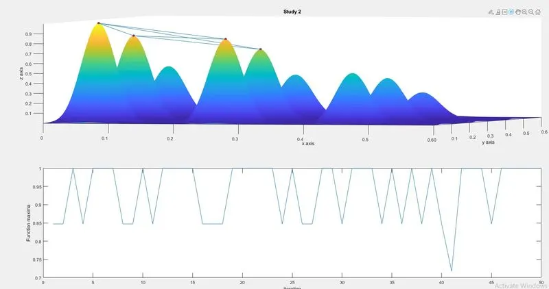
In here we again perform statistical behaviour with upper bound and lower bound ,upper bound and lower bounds helps to improve optimization .
As per compared to the first study 1 study 2 will be better result points are lowered and iteration will be optimize as compared to the first one.
In here upper bound and lower bound syntax will be different ,
x = ga(fun,nvars,A,b,Aeq,beq,lb,ub)
From this command fun is function which we named as stalagmite ,and nvars is number of design variables,
A,b is a linear equalities in which there is nothing so we can put it as blank so we give a [] for there ,
Aeq , beq are also linear equalities so here there is nothing so we can put [] for there,
lb and ub are the lower and upper bound so here it is 0 to 0.6 .
tic and toc command is used to get the study time taken for the ga to run and which is stored in Study2
 %plotting the data

 figure(2)
 subplot(2,1,1)
  hold on
 surfc(x,y,-f)
 shading interp
 xlabel('x axis')
 ylabel('y axis')
 zlabel('z axis')

  plot3(xopt2,yopt2,-fopt2,'marker','o','markerfacecolor','r','markersize',5)
 title('Study 2')
 subplot(2,1,2)
 plot(-fopt2)
 xlabel('Iteration')
 ylabel('Function maxima')
These command is used to plot the graph of the study 2.
%study3 GA Increasing Iteration

 options=optimoptions('ga');
 options=optimoptions(options,'populationsize',200);

 tic

 for r=1:num_cases
     [input,fopt3(r)]=ga(@stalagmite,2,[],[],[],[],[0,0],[0.6,0.6],[],[],options);
     xopt3(r)=input(1);
     yopt3(r)=input(2);

 end

 study3=toc
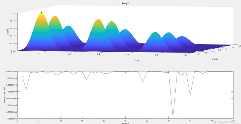
In here we have change in the syntax ga.In third study we use another constraint as options,it helps to increase the population to increase the size.
and we can see that the global maxima will be at top of function ,so the increase of population size we will get best results .
x = ga(fun,nvars,A,b,[],[],lb,ub,nonlcon,IntCon,options)
Here we use this syntax as we talk about above only few changes will occur in nonicon and Intcon these are the non linear equality constraints so we can give them as blank so we can give as [],[] .
 %plotting the data

 figure(3)
 subplot(2,1,1)
 hold on
 surf(x,y,-f)
 shading interp
 xlabel('x-axis')
 ylabel('y-axis')
 zlabel('Z-axis')


 plot3(xopt3,yopt3,-fopt3,'marker','o','markerfacecolor','r','markersize',5)
 title('Study 3')
 subplot(2,1,2)
  plot(-fopt3)
 xlabel('Iteration')
 ylabel('Function maxima')
These are the command for plotting the figure for the study 3.
Function Code Of Stalagmite:
function [f] = stalagmite(input_vector)
 x = input_vector(1);
 y = input_vector(2);

f1_x =(sin(5.1*pi*x+0.5))^6;
f1_y =(sin(5.1*pi*y+0.5))^6;

f2_x = exp(-4*log(2)*((x-0.0667)^2/0.64));
f2_y = exp(-4*log(2)*((y-0.0667)^2/0.64));

f =-[f1_x*f1_y*f2_x*f2_y];

end
In here we solve the equation in terms of f1_x,f1_y,f2_x,f2_y from these term f value is calculated so the value of f will store in the function and which goes to the main code .
Results:
Study 1
Study 2
Study 3
In this study we get the exact global maxima.
Conclusion:
To get the optimize value of global maxima we need to bound our inputs and also increase the iteration and increase population size