Week 4.1 - Genetic Algorithm

AIM: To write a code in MATLAB to optimise the stalagmite function and find the global maxima of the function.

THEORY:

GENETIC ALGORITHM

Algorithm is basically a process of natural selection that belongs to a big class of algorithms that have to be evolutionised.

Genetic algorithm (GA) is a method used to solve both constrained and unconstrained optimisation problems based on natural selection that is similar to that of biological evolution.It selects random individuals from the current generation to lead the evolution of the population to an optimal condition therefore, it keeps on modifying the a population of individual solutions. Genetic algorithm can be applied to solve problems that are suited for standard optimization algorithms,including problems in which the function is dicontinous,nondifferentiable,stochastic or highly non linear.

Firstly, before starting with the selection process, the ga starts with evaluating the fitness of each current member of the generation.This process is called fitness scaling.

Selection process:

Then, the members called as parents are selected on the basis of the above fitness scale score which contribute to the population of next gneration.

When two parents combine to form children for the next generation, the procees they undergo is called crossover and crossover rules are followed in this case.

Then , random changes are applied to the individual parents to form the children for the next generation which is based on the mutation rules.

TERMINATION OF GA:

The termination condition of a gais important for determining that when the process will end.Initially GA progresses very fast with better solutions coming in frequent iterations, but this trend slows down in the later stages where the improvements are very small.GA terminates when solution is close to the optimal, at the end of the run or any of the predefined criterias are almost met.

DEFINING THE FUNCTIONS:

FITNESS FUNCTION:

The fitness function is basically a function which takes the solution to a problem as input and returns a corresponding output value . It analyses how fit or appropriate the solution is to the given case problem.As we know from above explained selection process, fitness plays a key role in the process.

STALAGMITE FUNCTION:

function [F]= stalagmite_fun(input_vector)
x=input_vector(1);
y=input_vector(2);
f1=(sin((5.1*pi*x+0.5)))^6;
f2=((sin(5.1*pi*y+0.5)))^6;
f3= exp((-4*log(2)*((x-0.0667)^2)/0.64));
f4=exp((-4*log(2)*((y-0.0667)^2)/0.64));
F=(f1*f2*f3*f4*-1);
end

clear all
close all
clc
%defining search space
x=linspace(0,0.6,150);
y=linspace(0,0.6,150);
num_cases=50;
[xx, yy]=meshgrid(x,y);

%preparing the stalagmite function
for i=1:length(xx)
    for j=1:length(yy)
      input_vector(1)=xx(i,j);
      input_vector(2)=yy(i,j);
      f(i,j)=stalagmite_fun(input_vector);
    end
end

tic
%case1=Statistical behaviour
for k=1:num_cases
    [input,fopt(k)]=ga(@stalagmite_fun,2);
    xopt(k)=input(1);
    yopt(k)=input(2);
end
study_1=toc
figure(1)
subplot(2,1,1)
surfc(xx,yy,f)
hold on
plot3(xopt,yopt,fopt,'marker','o','markersize',5,'markerfacecolor','r');
title(' Unbounded Surface')
xlabel('xx value')
ylabel('yy value')
zlabel('ff value')
hold off
subplot(2,1,2)
plot(fopt)
title('Unbounded Surface study')
xlabel('Iteration')
ylabel('fopt1')
shading interp​

• Now, we proceed towards the first study case 1 of statistical behaviour in which, the number of cases taken are 50. Ga repeats itself for 50 times.
• The tic-toc command is used in order to find out the time taken for the program to finish.
• For loop command is then used and it's length is set as the number of cases.
• Then the ga command is used.
• Then the calculated optimum values are stored in the varibles xopt(k) and yopt(k) respectively.
• Then subplot command is used in order to get the plots in the same single figure.
• Using the surfc command ,xx,yy and f are plotted.
• Thereafter, titles and labels are given to the respective axes.
• Then, we plot the number of iterations against the function optimum(fopt) values.

%case2=Statistical behaviour with upper and lower bounds
tic
for k=1:num_cases
    [input,fopt(k)]=ga(@stalagmite_fun,2,[],[],[],[],[0;0],[0.6;0.6]);
    xopt(k)=input(1);
    yopt(k)=input(2);
end
study_2=toc
figure(2)
subplot(2,1,1)
surfc(xx,yy,f)
hold on
plot3(xopt,yopt,fopt,'marker','o','markersize',5,'markerfacecolor','r');
title('Bounded Surface')
xlabel('xx value')
ylabel('yy value')
zlabel('ff value')
hold off
subplot(2,1,2)
plot(fopt)
title('Bounded surface study')
xlabel('Iteration')
ylabel('fopt2')
shading interp

• In this part, we define a boundary for the ga to operate unlike in the first case where it has no boundaries of the search space
• All the commands in this study are similar to those explained in the case study 1 other than the syntax of ga command.
• In this program the lower limit is defined as 0,0 and upper limit is 0.6,0.6.
• Then, the plots are obtained in the same ,manner as we did in the above case.

%case3=Bounded optimized
options=optimoptions('ga');
options= optimoptions(options,'PopulationSize',400);

tic
for k=1:num_cases
    [input,fopt(k)]=ga(@stalagmite_fun,2,[],[],[],[],[0;0],[0.6;0.6],[],[],options);
    xopt(k)=input(1);
    yopt(k)=input(2);
end
study_3=toc
figure(3)
subplot(2,1,1)
surfc(xx,yy,f)
hold on
plot3(xopt,yopt,fopt,'marker','o','markersize',5,'markerfacecolor','r');
title('Bounded Surface with modified population size')
xlabel('xx value')
ylabel('yy value')
zlabel('ff value')
hold off
subplot(2,1,2)
plot(fopt)
title('Bounded surface study')
xlabel('Iteration')
ylabel('fopt3')
shading interp

• The commands used in case study 3 are similar to that explained in the case studies 1 and 2.
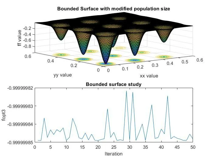
• In this case,other than setting the lower and upper boundaries ,iitial population six=ze is given for the ga to perform it's task.
• To set the initial population size,optimoptions command is used and then options and population size are mentioned.
• Then the plots are obtained in the same manner as we did in the prvious 2 case studies.

OBSERVATIONS:

• In the first case study(Statistical behaviour)a random value is obtained everytime and an exact global maxima value is not obtained.
• In the second study,the search space of ga is brought within the required boundary to overcome the problem faced in first case.But still, in the second study exact single global maxima value could not be obtained.
• So, in the third case,we set the population size for ga to operate and thus obtain a single point of global maximum could be found.

ERRORS:No errors were encountered during the working of the program.

RESULTS:

The time taken for each case study that was found out using the tic-toc command has returned the values as:

PLOTS:

FIGURE 1

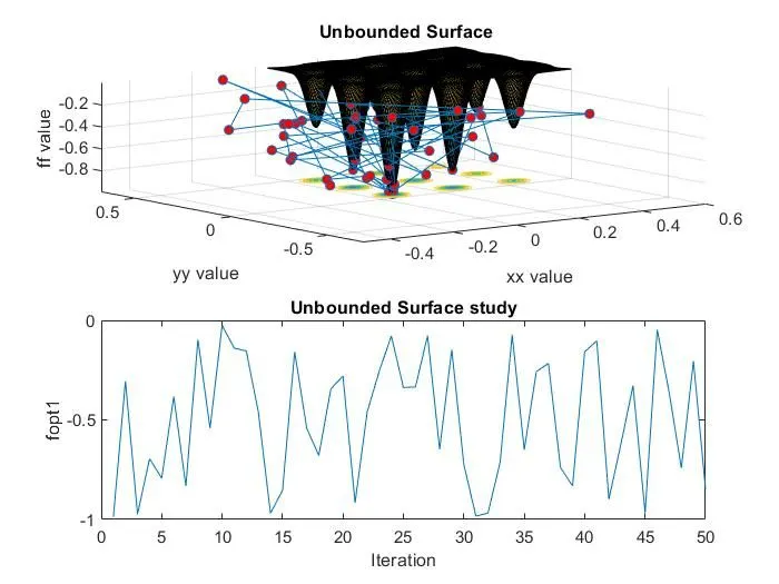
FIGURE 2

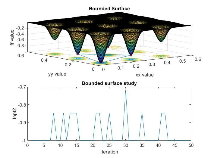
FIGURE 3

CONCLUSION:

• So as we can infer from this program we get an insight of how the ga works and its results vary when given different case scenarios and thus it's effect on the global maxima value.
• In the first case study,where the limits were unbounded, we were not able to obtain exact value.
• Whereas, in the third case when ga was given a boundary with defined population seze, it returned a much accurate global maxima value.

REFRENCES:

https://in.mathworks.com/help/gads/ga.html