Week 4.1 - Genetic Algorithm

Aim;

Write a code in MATLAB to optimise the stalagmite function and find the 'global maxima' of the function and plot graphs for all 3 studies and for F maximum vs no. of iterations.

Objectives;

The report is to optimize the Stalagmite function by coding the programe with help of Genetic Algorithm(ga) in MATLAB

Stalagmite;

A stalagmite is a type of rock formation that rises from the flooe=rof a cave due to the accumulationof the material deposited on the floor from the ceiling drippings. Stalagmite are typically compossed of calcium corbonate, but may consist of lava, mud, peat , pitch ,sand , sinter and ambreat.

Governing Equations for stalagmite function is;

f1(x)= [sin(5.1.pi.x+0.5]^6

f1(y)= [sin(5.1.pi.y+0.5]^6

f2(x) = exp(-4log2.(x-0.0667)^2)/0.64

f2(y) = exp(-4log2.(y-0.0667)^2)/0.64

f(xy) = f1(x).f1(y).f2(x).f2(y)

PROGRAM

The code for the stalagmite functoin;

function A = stalagmite(input_vector)
x= input_vector(1);
y= input_vector(2);
f1=(sin(5.1*pi*x+0.5)).^6;
f2=exp((-4*log(2)*((x-0.0667).^2))/0.64);
f3=(sin(5.1*pi*y+0.5)).^6;
f4=exp((-4*log(2))*((y-0.0667).^2)/0.64);
A=-(f1*f2*f3*f4);
end

Code for finding Global Maxima;

clear all
close all
clc
% search space
x = linspace(0,0.6,150);
y = linspace(0,0.6,150);

% creating 2-Dimensional mesh
[xx,yy] = meshgrid(x, y)

% evaluating the stalagmite function
for i = 1:length(xx)
    for j = 1:length(yy)
        input_vector(1)= xx(i,j);
        input_vector(2)= yy(i,j);
        f(i,j) = stalagmite(input_vector);
    end
end

% Converting fitting functions to change the dgraph upward
F = -f;

% ploting stalagmite function
surface(xx,yy,F);
shading interp;
hold on;

% performing the Generfic Algorithms
[output,fval] = ga(@stalagmite,2,[],[],[],[],[0,0],[0.6,0.6])

%ploting Global maxima
x_max = output(:,1);
y_max = output(:,2);
f_max = -fval;
plot3(x_max,y_max,f_max,'marker','o','markersize',5,'markerfacecolor','r');
xlabel('x-value');
ylabel('y-value');
title('GLOBAL MAXIMA');
legend('STALAGMITE','GLOBAL MAXIMA')

Result;

--------------------------------------------------------------------------------------------------------------------------------------------------------------

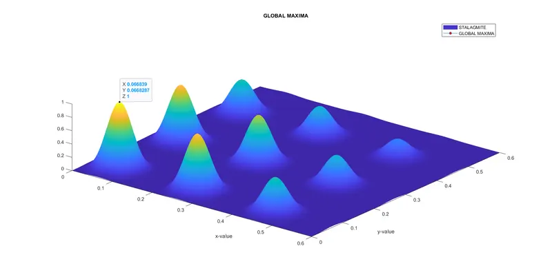
Code for Study-1, Statisficial Behaviour

close all
clear all
clc

x = linspace(0,0.6,150);
y = linspace(0,0.6,150);
num_case = 50;


% creating 2-Dimensional mesh
[xx,yy] = meshgrid(x, y);

% evaluating the stalagmite function
for i = 1:length(xx)
    for j = 1:length(yy)
        input_vector(1)= xx(i,j);
        input_vector(2)= yy(i,j);
        f(i,j) = stalagmite(input_vector);
    end
end
% converting Fitting function to change the graph upward
F = -f;

%performing the genetic algorithm
tic
for k = 1:num_case
    [inputs, fopt(k)]= ga(@stalagmite,2);
    xopt(k) = inputs(1);
    yopt(k) = inputs(2);
end

study_time = toc

%ploting Global maxima and function values
figure(1)
subplot(2,1,1)
hold on
surfc(x,y,F)
shading interp
plot3(xopt,yopt,-fopt,'marker','o','markersize',5,'markerfacecolor','r');
xlabel('x-value');
ylabel('y-value');
title('Unbounded Inputs');
legend('STALAGMITE','GLOBAL MAXIMA')
subplot(2,1,2)
hold on
plot(fopt)
xlabel('Iterations');
ylabel('Function Maxima');
title('variation in F');
legend('change in F value')

Results

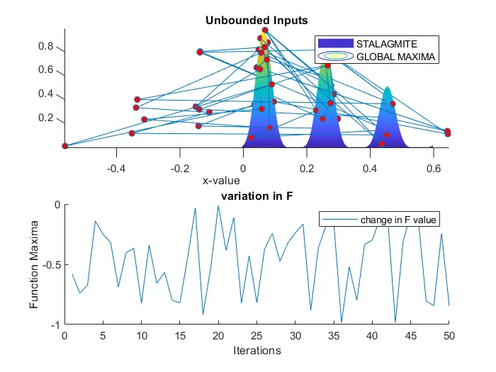
output =

0.0668 0.0668

fval =

-1.0000

-------------------------------------------------------------------------------------------------------------------------------------------------------------

Code for Study-2, Statistical Behaviour With Unbounded inputs and increased populations

clear all
close all
clc


x = linspace(0,0.6,150);
y = linspace(0,0.6,150);
num_case = 50;


% creating 2-Dimensional mesh
[xx,yy] = meshgrid(x, y);

% evaluating the stalagmite function
for i = 1:length(xx)
    for j = 1:length(yy)
        input_vector(1)= xx(i,j);
        input_vector(2)= yy(i,j);
        f(i,j) = stalagmite(input_vector);
    end
end
% converting Fitting function to change the graph upward
F = -f;

%performing the genetic algorithm
tic
for m = 1:num_case
    [inputs, fopt(m)]= ga(@stalagmite,2,[],[],[],[],[0,0],[0.6,0.6]);
    xopt(m) = inputs(1);
    yopt(m) = inputs(2);
end
fopt = -fopt;
study_time = toc

%ploting Global maxima and function values
figure(1)
subplot(2,1,1)
hold on
surfc(x,y,F)
shading interp
plot3(xopt,yopt,fopt,'marker','o','markersize',5,'markerfacecolor','r');
xlabel('x-value');
ylabel('y-value');
title('Unbounded Inputs');
legend('STALAGMITE','GLOBAL MAXIMA')
subplot(2,1,2)
hold on
plot(fopt)
xlabel('Iterations');
ylabel('Function Maxima');
title('variation in F');
legend('change in F value')

Results;

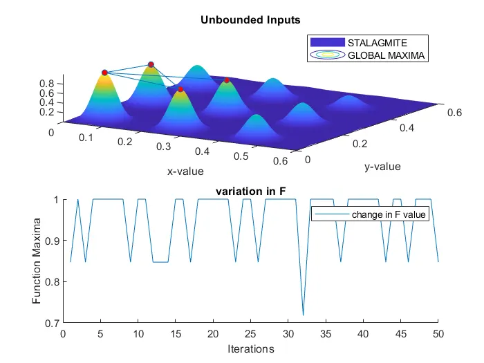
study_time =

4.0858

------------------------------------------------------------------------------------------------------------------------------------------------------

Code for Study-3, Statistical Behaviour With bounded inputs and increased populations

clear all
close all
clc



x = linspace(0,0.6,150);
y = linspace(0,0.6,150);
num_case = 50;


% creating 2-Dimensional mesh
[xx,yy] = meshgrid(x, y);

% evaluating the stalagmite function
for i = 1:length(xx)
    for j = 1:length(yy)
        input_vector(1)= xx(i,j);
        input_vector(2)= yy(i,j);
        f(i,j) = stalagmite(input_vector);
    end
end
% converting Fitting function to change the graph upward
F = -f;

%study 3 - increasing itration
options = optimoptions('ga');
options = optimoptions(options,'PopulationSize',600);


%performing the genetic algorithm
tic
for p = 1:num_case
    [inputs, fopt(p)]= ga(@stalagmite,2,[],[],[],[],[0,0],[0.1,0.1]);
    xopt(p) = inputs(1);
    yopt(p) = inputs(2);
end
fopt = -fopt;
study_time = toc

%ploting Global maxima and function values
figure(1)
subplot(2,1,1)
hold on
surfc(x,y,F)
shading interp
plot3(xopt,yopt,fopt,'marker','o','markersize',5,'markerfacecolor','r');
xlabel('x-value');
ylabel('y-value');
title('Unbounded Inputs');
legend('STALAGMITE','GLOBAL MAXIMA')
subplot(2,1,2)
hold on
plot(fopt)
xlabel('Iterations');
ylabel('Function Maxima');
title('F Maximum');
legend('change in F value')

Result

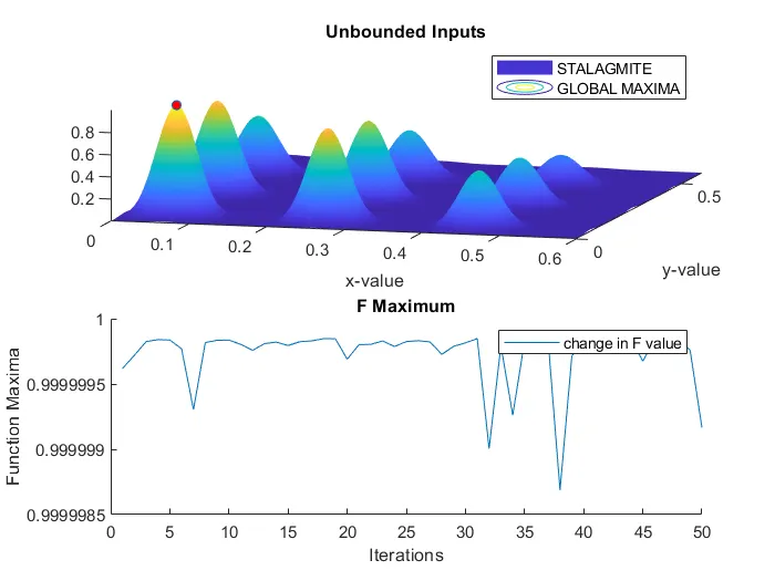
study_time =

8.2245